
Home > Article > Backend Development > In Python, images can be segmented and extracted using methods from the OpenCV library.

Segment or extract the foreground object in the image as the target image. The background itself is not interested. The watershed algorithm and the GrabCut algorithm segment and extract the image.
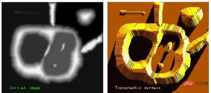
The watershed algorithm vividly compares images to geographical terrain surfaces to achieve image segmentation. This algorithm is very effective.
Any grayscale image can be regarded as a geographical terrain surface. Areas with high grayscale values can be regarded as mountain peaks. The grayscale value The lower areas can be thought of as valleys.
The left image is the original image, and the right image is its corresponding "topographic surface".
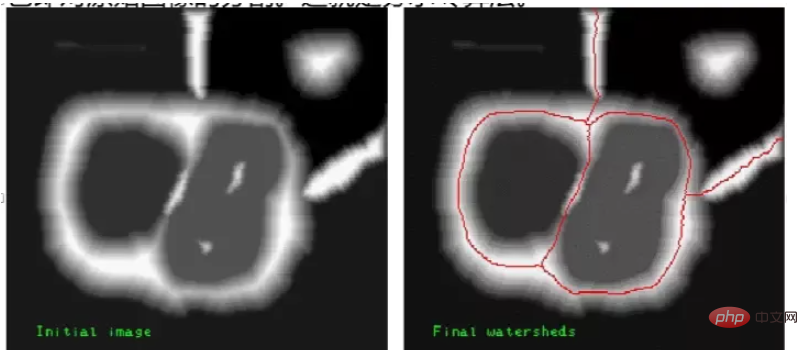
This process separates the image into two distinct sets: catchment basins and watershed lines. The dam we constructed is the watershed line, which is the segmentation of the original image. This is the watershed algorithm.
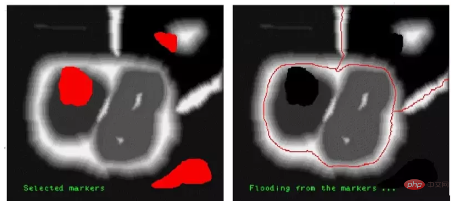
Due to the influence of noise and other factors, the above basic watershed algorithm often results in over-segmentation. Over-segmentation will divide the image into dense independent small blocks, making the segmentation meaningless. In order to improve the image segmentation effect, an improved mask-based watershed algorithm was proposed. The improved watershed algorithm allows the user to label parts that he thinks are the same segmented area (the labeled part is called a mask). When the watershed algorithm is processed, the marked parts will be processed into the same segmented area.
For example:
The original image is marked and processed, and three small color blocks marked as dark colors are represented. When using the mask watershed algorithm , the colors contained in these parts will be divided into the same area.
In OpenCV, you can use the function cv2.watershed() to implement the watershed algorithm.
In the specific implementation process, image segmentation needs to be completed with the help of morphological functions, distance transformation functions cv2.distanceTransform(), and cv2.connectedComponents().
Morphological function
Before using the watershed algorithm to segment the image, the image needs to be subjected to simple morphological processing.
Opening operation
Opening operation is an operation that corrodes first and then expands. Opening operation can remove the noise in the image
In processing with watershed algorithm Before image processing, the noise in the image must be removed using an opening operation to avoid possible interference caused by noise on image segmentation.
Get the image boundary
The boundary of the image can be obtained through morphological operations and subtraction operations.
Use morphological transformation to obtain the boundary information of an image
import cv2
import numpy as np
import matplotlib.pyplot as plt
o=cv2.imread("my.bmp", cv2.IMREAD_UNCHANGED)
k=np.ones((5,5), np.uint8)
e=cv2.erode(o, k)
b=cv2.subtract(o, e)
plt.subplot(131)
plt.imshow(o)
plt.axis('off')
plt.subplot(132)
plt.imshow(e)
plt.axis('off')
plt.subplot(133)
plt.imshow(b)
plt.axis('off')
plt.show()
Use morphological operations and subtraction operations to obtain the boundary information of the image. However, morphological operations are only suitable for relatively simple images. If the foreground objects in the image are connected, the boundaries of each sub-image cannot be accurately obtained using morphological operations.
Distance transformation function distanceTransform
When the sub-images in the image are not connected, the morphological erosion operation can be used directly to determine the foreground object, but if the sub-images in the image are connected When they are together, it is difficult to determine the foreground object
At this time, the foreground object can be easily extracted with the help of the distance transformation function cv2.distanceTransform().
The function cv2.distanceTransform() calculates the distance from any point in the binary image to the nearest background point.
Generally, this function calculates the distance from a non-zero value pixel in the image to the nearest zero-value pixel, that is, it calculates the distance between all pixels in the binary image and its nearest pixel with a value of 0. .
If the value of the pixel itself is 0, then the distance is also 0.
The calculation result of cv2.distanceTransform() reflects the distance relationship between each pixel and the background (pixel point with value 0).
Normally:
If the center (center of mass) of the foreground object is 0 pixel distance away The farther you go, the larger the value will be.
If the edge of the foreground object is closer to the pixel with a value of 0, a smaller value will be obtained.
If the above calculation results are thresholded, the center, skeleton and other information of the sub-image within the image can be obtained. The distance transformation function cv2.distanceTransform() can be used to calculate the center of the object, and can also refine the outline, obtain the image foreground, etc.
The syntax format of the function cv2.distanceTransform() is:
dst=cv2.distanceTransform(src, distanceType, maskSize[, dstType]])
src is an 8-bit single-channel binary image.
distanceType is the distance type parameter
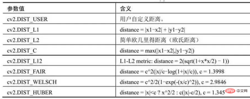
maskSize为掩模的尺寸
distanceType=cv2.DIST_L1或cv2.DIST_C时,maskSize强制为3(因为设置为3和设置为5及更大值没有什么区别)。
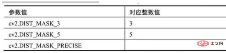
dstType为目标图像的类型,默认值为CV_32F。
dst表示计算得到的目标图像,可以是8位或32位浮点数,尺寸和src相同。
使用距离变换函数cv2.distanceTransform(),计算一幅图像的确定前景
import numpy as np
import cv2
import matplotlib.pyplot as plt
img = cv2.imread('water_coins.jpg')
gray = cv2.cvtColor(img, cv2.COLOR_BGR2GRAY)

img=cv2.cvtColor(img, cv2.COLOR_BGR2RGB)
ishow=img.copy()
ret, thresh = cv2.threshold(gray,0,255,cv2.THRESH_BINARY_INV+cv2.THRESH_OTSU)
kernel = np.ones((3,3), np.uint8)
opening = cv2.morphologyEx(thresh, cv2.MORPH_OPEN, kernel, iterations = 2) # 进行开运算
dist_transform = cv2.distanceTransform(opening, cv2.DIST_L2,5)
ret, fore = cv2.threshold(dist_transform,0.7*dist_transform.max(),255,0)
plt.subplot(131)
plt.imshow(ishow)
plt.axis('off')
plt.subplot(132)
plt.imshow(dist_transform)
plt.axis('off')
plt.subplot(133)
plt.imshow(fore)
plt.axis('off')
plt.show()
fore图像中: 比较准确地显示出左图内的“确定前景”。确定前景,通常是指前景对象的中心。之所以认为这些点是确定前景,是因为它们距离背景点的距离足够远,都是距离大于足够大的固定阈值(0.7*dist_transform.max())的点。
确定未知区域
使用形态学的膨胀操作能够将图像内的前景“膨胀放大”。
当图像内的前景被放大后,背景就会被“压缩”,所以此时得到的背景信息一定小于实际背景的,不包含前景的“确定背景”。
为了方便说明将确定背景称为B。
距离变换函数cv2.distanceTransform()能够获取图像的“中心”,得到“确定前景”。
图像中有了确定前景F和确定背景B,剩下区域的就是未知区域UN了。这部分区域正是分水岭算法要进一步明确的区域。
针对一幅图像O,通过以下关系能够得到未知区域UN:
未知区域UN=图像O-确定背景B-确定前景F
未知区域UN=(图像O-确定背景B)- 确定前景F
“图像O-确定背景B”,可以通过对图像进行形态学的膨胀操作得到。
标注一幅图像的确定前景、确定背景及未知区域。
import numpy as np
import cv2
import matplotlib.pyplot as plt
img = cv2.imread('water_coins.jpg')
gray = cv2.cvtColor(img, cv2.COLOR_BGR2GRAY)
img=cv2.cvtColor(img, cv2.COLOR_BGR2RGB)
ishow=img.copy()
ret, thresh = cv2.threshold(gray,0,255,cv2.THRESH_BINARY_INV+cv2.THRESH_OTSU)
kernel = np.ones((3,3), np.uint8)
opening = cv2.morphologyEx(thresh, cv2.MORPH_OPEN, kernel, iterations = 2)
bg = cv2.dilate(opening, kernel, iterations=3)
dist = cv2.distanceTransform(opening, cv2.DIST_L2,5)
ret, fore = cv2.threshold(dist,0.7*dist.max(),255,0)
fore = np.uint8(fore)
un = cv2.subtract(bg, fore)
plt.subplot(221)
plt.imshow(ishow)
plt.axis('off')
plt.subplot(222)
plt.imshow(bg)
plt.axis('off')
plt.subplot(223)
plt.imshow(fore)
plt.axis('off')
plt.subplot(224)
plt.imshow(un)
plt.axis('off')
plt.show()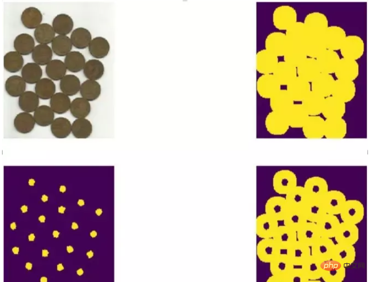
函数connectedComponents
明确了确定前景后,就可以对确定前景图像进行标注了。
在OpenCV中,可以使用函数cv2.connectedComponents()进行标注。该函数会将背景标注为0,将其他的对象使用从1开始的正整数标注。
函数cv2.connectedComponents()的语法格式为:
retval, labels = cv2.connectedComponents( image )
image为8位单通道的待标注图像。
retval为返回的标注的数量。
labels为标注的结果图像。
使用函数cv2.connectedComponents()标注一幅图像
import numpy as np
import cv2
import matplotlib.pyplot as plt
img = cv2.imread('water_coins.jpg')
gray = cv2.cvtColor(img, cv2.COLOR_BGR2GRAY)
img=cv2.cvtColor(img, cv2.COLOR_BGR2RGB)
ishow=img.copy()
ret, thresh = cv2.threshold(gray,0,255,cv2.THRESH_BINARY_INV+cv2.THRESH_OTSU)
kernel = np.ones((3,3), np.uint8)
opening = cv2.morphologyEx(thresh, cv2.MORPH_OPEN, kernel, iterations = 2)
sure_bg = cv2.dilate(opening, kernel, iterations=3)
dist_transform = cv2.distanceTransform(opening, cv2.DIST_L2,5)
ret, fore = cv2.threshold(dist_transform,0.7*dist_transform.max(),255,0)
fore = np.uint8(fore)
ret, markers = cv2.connectedComponents(fore)
print(ret)
plt.subplot(131)
plt.imshow(ishow)
plt.axis('off')
plt.subplot(132)
plt.imshow(fore)
plt.axis('off')
plt.subplot(133)
plt.imshow(markers)
plt.axis('off')
plt.show()
前景图像的中心点被做了不同的标注(用不同颜色区分)
函数cv2.connectedComponents()在标注图像时,会将背景标注为0,将其他的对象用从1开始的正整数标注。具体的对应关系为:
数值0代表背景区域。
从数值1开始的值,代表不同的前景区域。
在分水岭算法中,标注值0代表未知区域。所以,我们要对函数cv2.connectedComponents()标注的结果进行调整:将标注的结果都加上数值1。经过上述处理后,在标注结果中:
数值1代表背景区域。
从数值2开始的值,代表不同的前景区域。
为了能够使用分水岭算法,还需要对原始图像内的未知区域进行标注,将已经计算出来的未知区域标注为0即可。
关键代码:
ret, markers = cv2.connectedComponents(fore)
markers = markers+1
markers[未知区域] = 0
使用函数cv2.connectedComponents()标注一幅图像,并对其进行修正,使未知区域被标注为0
import numpy as np
import cv2
import matplotlib.pyplot as plt
img = cv2.imread('water_coins.jpg')
gray = cv2.cvtColor(img, cv2.COLOR_BGR2GRAY)
img=cv2.cvtColor(img, cv2.COLOR_BGR2RGB)
ishow=img.copy()
ret, thresh = cv2.threshold(gray,0,255,cv2.THRESH_BINARY_INV+cv2.THRESH_OTSU)
kernel = np.ones((3,3), np.uint8)
opening = cv2.morphologyEx(thresh, cv2.MORPH_OPEN, kernel, iterations = 2)
sure_bg = cv2.dilate(opening, kernel, iterations=3)
dist_transform = cv2.distanceTransform(opening, cv2.DIST_L2,5)
ret, fore = cv2.threshold(dist_transform,0.7*dist_transform.max(),255,0)
fore = np.uint8(fore)
ret, markers1 = cv2.connectedComponents(fore)
foreAdv=fore.copy()
unknown = cv2.subtract(sure_bg, foreAdv)
ret, markers2 = cv2.connectedComponents(foreAdv)
markers2 = markers2+1
markers2[unknown==255] = 0
plt.subplot(121)
plt.imshow(markers1)
plt.axis('off')
plt.subplot(122)
plt.imshow(markers2)
plt.axis('off')
plt.show()
前景都有一个黑色的边缘,这个边缘是被标注的未知区域。
函数cv2.watershed()
完成上述处理后,就可以使用分水岭算法对预处理结果图像进行分割了。
在OpenCV中,实现分水岭算法的函数是cv2.watershed(),其语法格式为:
markers = cv2.watershed( image, markers )
image是输入图像,必须是8位三通道的图像。在对图像使用
cv2.watershed()函数处理之前,必须先用正数大致勾画出图像中的期望分割区域。每一个分割的区域会被标注为1、2、3等。对于尚未确定的区域,需要将它们标注为0。我们可以将标注区域理解为进行分水岭算法分割的“种子”区域。
markers是32位单通道的标注结果,它应该和image具有相等大小。在markers中,每一个像素要么被设置为初期的“种子值”,要么被设置为**“-1”表示边界**。
使用分水岭算法进行图像分割时,基本的步骤为:
通过形态学开运算对原始图像O去噪。
通过腐蚀操作获取“确定背景B”。
需要注意,这里得到“原始图像-确定背景”即可。
利用距离变换函数cv2.distanceTransform()对原始图像进行运算,并对其进行阈值处理,得到“确定前景F”。
计算未知区域UN(UN=O -B - F)
利用函数cv2.connectedComponents()对原始图像O进行标注。
对函数cv2.connectedComponents()的标注结果进行修正。
使用分水岭函数完成对图像的分割。
使用分水岭算法对一幅图像进行分割:
import numpy as np
import cv2
import matplotlib.pyplot as plt
img = cv2.imread('water_coins.jpg')
gray = cv2.cvtColor(img, cv2.COLOR_BGR2GRAY)
img=cv2.cvtColor(img, cv2.COLOR_BGR2RGB)
ishow=img.copy()
ret, thresh = cv2.threshold(gray,0,255,cv2.THRESH_BINARY_INV+cv2.THRESH_OTSU)
kernel = np.ones((3,3), np.uint8)
opening = cv2.morphologyEx(thresh, cv2.MORPH_OPEN, kernel, iterations = 2)
sure_bg = cv2.dilate(opening, kernel, iterations=3)
dist_transform = cv2.distanceTransform(opening, cv2.DIST_L2,5)
ret, sure_fg = cv2.threshold(dist_transform,0.7*dist_transform.max(),255,0)
sure_fg = np.uint8(sure_fg)
unknown = cv2.subtract(sure_bg, sure_fg)
ret, markers = cv2.connectedComponents(sure_fg)
markers = markers+1
markers[unknown==255] = 0
markers = cv2.watershed(img, markers)
img[markers == -1] = [0,255,0] # 边界
plt.subplot(121)
plt.imshow(ishow)
plt.axis('off')
plt.subplot(122)
plt.imshow(img)
plt.axis('off')
plt.show()经典的前景提取技术主要使用纹理(颜色)信息,如魔术棒工具,或根据边缘(对比度)信息,如智能剪刀等。在开始提取前景时,先用一个矩形框指定前景区域所在的大致位置范围,然后不断迭代地分割,直到达到最好的效果。经过上述处理后,提取前景的效果可能并不理想,存在前景没有提取出来,或者将背景提取为前景的情况,此时需要用户干预提取过程。
用户在原始图像的副本中(也可以是与原始图像大小相等的任意一幅图像),用白色标注要提取为前景的区域,用黑色标注要作为背景的区域。然后,将标注后的图像作为掩模,让算法继续迭代提取前景从而得到最终结果。
GrabCut算法的具体实施过程。
将前景所在的大致位置使用矩形框标注出来。
此时矩形框框出的仅仅是前景的大致位置,其中既包含前景又包含背景,所以该区域实际上是未确定区域。但是,该区域以外的区域被认为是“确定背景”。
根据矩形框外部的“确定背景”数据来区分矩形框区域内的前景和背景。
用高斯混合模型(Gaussians Mixture Model, GMM)对前景和背景建模。
GMM会根据用户的输入 学习并创建新的像素分布。对未分类的像素(可能是背景也可能是前景),根据其与已知分类像素(前景和背景)的关系进行分类。
根据像素分布情况生成一幅图,图中的节点就是各个像素点。
除了像素点之外,还有两个节点:前景节点和背景节点。所有的前景像素都和前景节点相连,所有的背景像素都和背景节点相连。每个像素连接到前景节点或背景节点的边的权重由像素是前景或背景的概率来决定。
图中的每个像素除了与前景节点或背景节点相连外,彼此之间还存在着连接。两个像素连接的边的权重值由它们的相似性决定,两个像素的颜色越接近,边的权重值越大。
完成节点连接后,需要解决的问题变成了一幅连通的图。在该图上根据各自边的权重关系进行切割,将不同的点划分为前景节点和背景节点。
不断重复上述过程,直至分类收敛为止。
在OpenCV中,实现交互式前景提取的函数是cv2.grabCut(),其语法格式为:
mask, bgdModel, fgdModel =cv2.grabCut(img, mask, rect, bgdModel, fgdModel, iterCount[, mode] )
img为输入图像,要求是8位3通道的。
mask为掩模图像,要求是8位单通道的。该参数用于确定前景区域、背景区域和不确定区域,可以设置为4种形式。
cv2.GC_BGD:表示确定背景,也可以用数值0表示。
cv2.GC_FGD:表示确定前景,也可以用数值1表示。
cv2.GC_PR_BGD:表示可能的背景,也可以用数值2表示。
cv2.GC_PR_FGD:表示可能的前景,也可以用数值3表示。
在最后使用模板提取前景时,会将参数值0和2合并为背景(均当作0处理),将参数值1和3合并为前景(均当作1处理)。
在通常情况下,我们可以使用白色笔刷和黑色笔刷在掩模图像上做标记,再通过转换将其中的白色像素设置为0,黑色像素设置为1。
rect指包含前景对象的区域,该区域外的部分被认为是“确定背景”。因此,在选取时务必确保让前景包含在rect指定的范围内;否则,rect外的前景部分是不会被提取出来的。
只有当参数mode的值被设置为矩形模式cv2.GC_INIT_WITH_RECT时,参数rect才有意义。
其格式为(x, y, w, h),分别表示区域左上角像素的x轴和y轴坐标以及区域的宽度和高度。
如果前景位于右下方,又不想判断原始图像的大小,对于w 和h可以直接用一个很大的值。
使用掩模模式时,将该值设置为none即可。
bgdModel为算法内部使用的数组,只需要创建大小为(1, 65)的numpy.float64数组。
fgdModel为算法内部使用的数组,只需要创建大小为(1, 65)的numpy.float64数组。
iterCount表示迭代的次数。
mode表示迭代模式。其可能的值与含义如下:
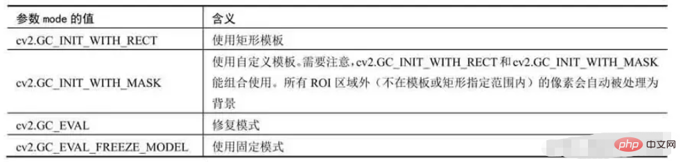
RECT 和MASK可以组合使用( 并的关系 )
使用GrabCut算法提取图像的前景
import numpy as np
import cv2
import matplotlib.pyplot as plt
o = cv2.imread('lenacolor.png')
orgb=cv2.cvtColor(o, cv2.COLOR_BGR2RGB)
mask = np.zeros(o.shape[:2], np.uint8)
bgdModel = np.zeros((1,65), np.float64)
fgdModel = np.zeros((1,65), np.float64)
rect = (50,50,400,500)
cv2.grabCut(o, mask, rect, bgdModel, fgdModel,5, cv2.GC_INIT_WITH_RECT)
mask2 = np.where((mask==2)|(mask==0),0,1).astype('uint8')
ogc = o*mask2[:, :, np.newaxis]
ogc=cv2.cvtColor(ogc, cv2.COLOR_BGR2RGB)
plt.subplot(121)
plt.imshow(orgb)
plt.axis('off')
plt.subplot(122)
plt.imshow(ogc)
plt.axis('off')
plt.show()
为了得到完整的前景对象,需要做一些改进。
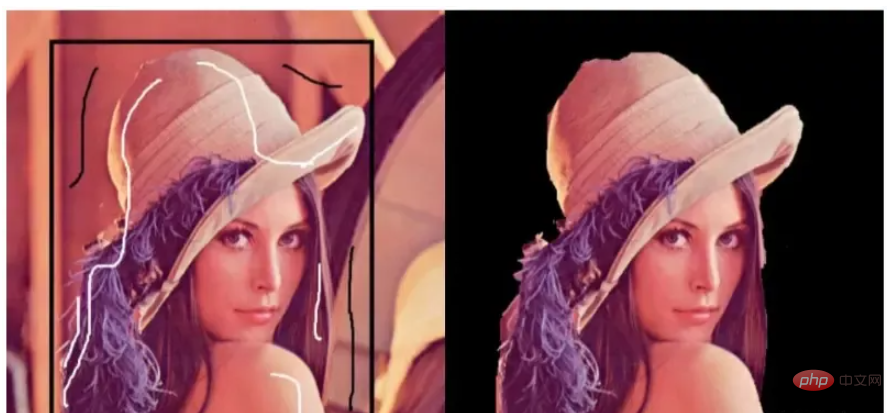
这里对原始图像进行标注,将需要保留的部分设置为白色,将需要删除的背景设置为黑色。以标记好的图像作为模板,使用函数cv2.grabCut()完成前景的提取。
这个过程主要包含以下步骤:
利用函数cv2.grabCut()在cv2.GC_INIT_WITH_RECT 模式下对图像进行初步的前景提取,得到初步提取的结果图像og。
使用Windows系统自带的笔刷工具,打开要提取前景的图像,比如lena。
使用白色笔刷在希望提取的前景区域做标记。
使用黑色笔刷在希望删除的背景区域做标记。
将当前设置好的lena图像另存为模板图像m0。
将模板图像m0中的白色值和黑色值映射到模板m中。将模板图像m0中的白色值(像素值为255)映射为模板图像m中的确定前景(像素值为1),将模板图像m0中的黑色值(像素值为0)映射为模板图像m中的确定背景(像素值为0)。
以模板图像m作为函数cv2.grabCut()的模板参数(mask),对图像og完成前景提取。
使用画笔标记的模板图像m0不能直接作为模板(即参数mask)使用
函数cv2.grabCut()要求,参数mask的值必须是cv2.GC_BGD(确定背景)、cv2.GC_FGD(确定前景)、cv2.GC_PR_BGD(可能的背景)、cv2.GC_PR_FGD(可能的前景),或者是0、1、2、3之中的值。
必须先将模板图像m0中的白色值和黑色值映射到模板m上,再将模板图像m作为函数cv2.grabCut()的模板参数。
在GrabCut算法中使用模板提取图像的前景:
import numpy as np
import cv2
import matplotlib.pyplot as plt
o= cv2.imread('lenacolor.png')
orgb=cv2.cvtColor(o, cv2.COLOR_BGR2RGB)
mask = np.zeros(o.shape[:2], np.uint8)
bgd = np.zeros((1,65), np.float64)
fgd = np.zeros((1,65), np.float64)
rect = (50,50,400,500)
cv2.grabCut(o, mask, rect, bgd, fgd,5, cv2.GC_INIT_WITH_RECT)
mask2 = cv2.imread('mask.png',0)
mask2Show = cv2.imread('mask.png', -1)
m2rgb=cv2.cvtColor(mask2Show, cv2.COLOR_BGR2RGB)
mask[mask2 == 0] = 0
mask[mask2 == 255] = 1
mask, bgd, fgd = cv2.grabCut(o, mask, None, bgd, fgd,5, cv2.GC_INIT_WITH_MASK)
mask = np.where((mask==2)|(mask==0),0,1).astype('uint8')
ogc = o*mask[:, :, np.newaxis]
ogc=cv2.cvtColor(ogc, cv2.COLOR_BGR2RGB)
plt.subplot(121)
plt.imshow(m2rgb)
plt.axis('off')
plt.subplot(122)
plt.imshow(ogc)
plt.axis('off')
plt.show()
在函数cv2.grabCut()的实际使用中,也可以不使用矩形初始化,直接使用模板模式。构造一个模板图像,其中:
使用像素值0标注确定背景。
使用像素值1标注确定前景。
使用像素值2标注可能的背景。
使用像素值3标注可能的前景。
构造完模板后,直接将该模板用于函数cv2.grabCut()处理原始图像,即可完成前景的提取。
一般情况下,自定义模板的步骤为:
先使用numpy.zeros构造一个内部像素值都是0(表示确定背景)的图像mask,以便在后续步骤中逐步对该模板图像进行细化。
.使用mask[30:512, 50:400]=3,将模板图像中第30行到第512行,第50列到400列的区域划分为可能的前景(像素值为3,对应参数mask的含义为“可能的前景”)。
使用mask[50:300, 150:200]=1,将模板图像中第50行到第300行,第150列到第200列的区域划分为确定前景(像素值为1,对应参数mask的含义为“确定前景”)。
在GrabCut算法中直接使用自定义模板提取图像的前景
import numpy as np
import cv2
import matplotlib.pyplot as plt
o= cv2.imread('lenacolor.png')
orgb=cv2.cvtColor(o, cv2.COLOR_BGR2RGB)
bgd = np.zeros((1,65), np.float64)
fgd = np.zeros((1,65), np.float64)
mask2 = np.zeros(o.shape[:2], np.uint8)
#先将掩模的值全部构造为0(确定背景),在后续步骤中,再根据需要修改其中的部分值
mask2[30:512,50:400]=3 #lena头像的可能区域
mask2[50:300,150:200]=1 #lena头像的确定区域,如果不设置这个区域,头像的提取不完整
cv2.grabCut(o, mask2, None, bgd, fgd,5, cv2.GC_INIT_WITH_MASK)
mask2 = np.where((mask2==2)|(mask2==0),0,1).astype('uint8')
ogc = o*mask2[:, :, np.newaxis]
ogc=cv2.cvtColor(ogc, cv2.COLOR_BGR2RGB)
plt.subplot(121)
plt.imshow(orgb)
plt.axis('off')
plt.subplot(122)
plt.imshow(ogc)
plt.axis('off')
plt.show()
对于不同的图像,要构造不同的模板来划分它们的确定前景、确定背景、可能的前景与可能的背景。
The above is the detailed content of In Python, images can be segmented and extracted using methods from the OpenCV library.. For more information, please follow other related articles on the PHP Chinese website!