Example of building a simple neural network on PyTorch to implement regression and classification

This article mainly introduces examples of building a simple neural network on PyTorch to implement regression and classification. Now I share it with you and give it as a reference. Let’s take a look together

This article introduces an example of building a simple neural network on PyTorch to implement regression and classification. I would like to share it with you. The details are as follows:

1. Getting started with PyTorch

1. Installation method

Log in to the PyTorch official website, http://pytorch.org, you can See the following interface:

After selecting the option in the picture above, you can get the conda command under Linux:

conda install pytorch torchvision -c soumith

Currently PyTorch only supports MacOS and Linux, and does not support Windows yet. Installing PyTorch will install two modules, one is torch and the other is torchvision. Torch is the main module, which is used to build neural networks. torchvision is the auxiliary module, which has a database and some already trained neural networks waiting for you to use directly. For example (VGG, AlexNet, ResNet).

2. Numpy and Torch

torch_data = torch.from_numpy(np_data) can convert numpy(array) format to torch(tensor) format; torch_data.numpy( ) can also convert the tensor format of torch to the array format of numpy. Note that Torch's Tensor and numpy's array will share their storage space, and modifying one will cause the other to be modified.

For 1-dimensional (1-D) data, numpy prints output in the form of row vectors, while torch prints output in the form of column vectors.

Other functions in numpy such as sin, cos, abs, mean, etc. can be used in the same way in torch. It should be noted that matrix multiplication of np.matmul(data, data) and data.dot(data) in numpy will yield the same result; torch.mm(tensor, tensor) in torch is a matrix multiplication method, resulting in a matrix , tensor.dot(tensor) will convert the tensor into a 1-dimensional tensor, then multiply it element by element and sum it up to get a real number.

Related code:

import torch 
import numpy as np 
 
np_data = np.arange(6).reshape((2, 3)) 
torch_data = torch.from_numpy(np_data) # 将numpy(array)格式转换为torch(tensor)格式 
tensor2array = torch_data.numpy()  
print( 
  '\nnumpy array:\n', np_data,  
  '\ntorch tensor:', torch_data,  
  '\ntensor to array:\n', tensor2array,  
) # torch数据格式在print的时候前后自动添加换行符 
 
# abs 
data = [-1, -2, 2, 2] 
tensor = torch.FloatTensor(data)  
print( 
  '\nabs', 
  '\nnumpy: \n', np.abs(data),     
  '\ntorch: ', torch.abs(tensor)  
) # 1维的数据，numpy是行向量形式显示，torch是列向量形式显示 
 
# sin 
print( 
  '\nsin', 
  '\nnumpy: \n', np.sin(data),    
  '\ntorch: ', torch.sin(tensor)  
) 
 
# mean 
print( 
  '\nmean', 
  '\nnumpy: ', np.mean(data),   
  '\ntorch: ', torch.mean(tensor)  
) 
 
# 矩阵相乘 
data = [[1,2], [3,4]] 
tensor = torch.FloatTensor(data)  
 
print( 
  '\nmatrix multiplication (matmul)', 
  '\nnumpy: \n', np.matmul(data, data),   
  '\ntorch: ', torch.mm(tensor, tensor)  
) 
 
data = np.array(data) 
print( 
  '\nmatrix multiplication (dot)', 
  '\nnumpy: \n', data.dot(data),    
  '\ntorch: ', tensor.dot(tensor)   
)

##3. Variable

PyTorch The neural network in comes from the autograd package, which provides automatic derivation methods for all operations of Tensor.

autograd.Variable This is the core class in this package. Variable can be understood as a container containing tensor, which wraps a Tensor and supports almost all operations defined on it. Once the operation is completed, .backward() can be called to automatically calculate all gradients. In other words, only by placing the tensor in Variable can operations such as reverse transfer and automatic derivation be implemented in the neural network.

The original tensor can be accessed through the attribute .data, and the gradient of this Variable can be viewed through the .grad attribute.

Related codes:

import torch 
from torch.autograd import Variable 
 
tensor = torch.FloatTensor([[1,2],[3,4]]) 
variable = Variable(tensor, requires_grad=True) 
# 打印展示Variable类型 
print(tensor) 
print(variable) 
 
t_out = torch.mean(tensor*tensor) # 每个元素的^ 2 
v_out = torch.mean(variable*variable) 
print(t_out) 
print(v_out) 
 
v_out.backward() # Variable的误差反向传递 
 
# 比较Variable的原型和grad属性、data属性及相应的numpy形式 
print('variable:\n', variable) 
# v_out = 1/4 * sum(variable*variable) 这是计算图中的 v_out 计算步骤 
# 针对于 v_out 的梯度就是, d(v_out)/d(variable) = 1/4*2*variable = variable/2 
print('variable.grad:\n', variable.grad) # Variable的梯度 
print('variable.data:\n', variable.data) # Variable的数据 
print(variable.data.numpy()) #Variable的数据的numpy形式

##Partial output results:

variable:

Variable containing:

1 2
3 4
[torch.FloatTensor of size 2x2]
variable.grad:
Variable containing:
0.5000 1.0000
1.5000 2.0000
[torch.FloatTensor of size 2x2]
variable.data:
1 2
3 4
[torch.FloatTensor of size 2x2]
[[ 1 . 2.]
[ 3. 4.]]

4. Activation function activationfunction

Torch’s activation functions are all in torch.nn. In functional, relu, sigmoid, tanh, softplus are all commonly used excitation functions.

Related codes:

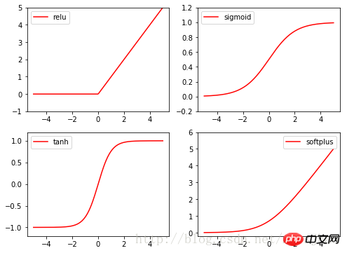
import torch 
import torch.nn.functional as F 
from torch.autograd import Variable 
import matplotlib.pyplot as plt 
 
x = torch.linspace(-5, 5, 200) 
x_variable = Variable(x) #将x放入Variable 
x_np = x_variable.data.numpy() 
 
# 经过4种不同的激励函数得到的numpy形式的数据结果 
y_relu = F.relu(x_variable).data.numpy() 
y_sigmoid = F.sigmoid(x_variable).data.numpy() 
y_tanh = F.tanh(x_variable).data.numpy() 
y_softplus = F.softplus(x_variable).data.numpy() 
 
plt.figure(1, figsize=(8, 6)) 
 
plt.subplot(221) 
plt.plot(x_np, y_relu, c='red', label='relu') 
plt.ylim((-1, 5)) 
plt.legend(loc='best') 
 
plt.subplot(222) 
plt.plot(x_np, y_sigmoid, c='red', label='sigmoid') 
plt.ylim((-0.2, 1.2)) 
plt.legend(loc='best') 
 
plt.subplot(223) 
plt.plot(x_np, y_tanh, c='red', label='tanh') 
plt.ylim((-1.2, 1.2)) 
plt.legend(loc='best') 
 
plt.subplot(224) 
plt.plot(x_np, y_softplus, c='red', label='softplus') 
plt.ylim((-0.2, 6)) 
plt.legend(loc='best') 
 
plt.show()

##2. PyTorch implements regression

Look at the complete code first:

import torch 
from torch.autograd import Variable 
import torch.nn.functional as F 
import matplotlib.pyplot as plt 
 
x = torch.unsqueeze(torch.linspace(-1, 1, 100), dim=1) # 将1维的数据转换为2维数据 
y = x.pow(2) + 0.2 * torch.rand(x.size()) 
 
# 将tensor置入Variable中 
x, y = Variable(x), Variable(y) 
 
#plt.scatter(x.data.numpy(), y.data.numpy()) 
#plt.show() 
 
# 定义一个构建神经网络的类 
class Net(torch.nn.Module): # 继承torch.nn.Module类 
  def __init__(self, n_feature, n_hidden, n_output): 
    super(Net, self).__init__() # 获得Net类的超类（父类）的构造方法 
    # 定义神经网络的每层结构形式 
    # 各个层的信息都是Net类对象的属性 
    self.hidden = torch.nn.Linear(n_feature, n_hidden) # 隐藏层线性输出 
    self.predict = torch.nn.Linear(n_hidden, n_output) # 输出层线性输出 
 
  # 将各层的神经元搭建成完整的神经网络的前向通路 
  def forward(self, x): 
    x = F.relu(self.hidden(x)) # 对隐藏层的输出进行relu激活 
    x = self.predict(x) 
    return x 
 
# 定义神经网络 
net = Net(1, 10, 1) 
print(net) # 打印输出net的结构 
 
# 定义优化器和损失函数 
optimizer = torch.optim.SGD(net.parameters(), lr=0.5) # 传入网络参数和学习率 
loss_function = torch.nn.MSELoss() # 最小均方误差 
 
# 神经网络训练过程 
plt.ion()  # 动态学习过程展示 
plt.show() 
 
for t in range(300): 
  prediction = net(x) # 把数据x喂给net，输出预测值 
  loss = loss_function(prediction, y) # 计算两者的误差，要注意两个参数的顺序 
  optimizer.zero_grad() # 清空上一步的更新参数值 
  loss.backward() # 误差反相传播，计算新的更新参数值 
  optimizer.step() # 将计算得到的更新值赋给net.parameters() 
 
  # 可视化训练过程 
  if (t+1) % 10 == 0: 
    plt.cla() 
    plt.scatter(x.data.numpy(), y.data.numpy()) 
    plt.plot(x.data.numpy(), prediction.data.numpy(), 'r-', lw=5) 
    plt.text(0.5, 0, 'L=%.4f' % loss.data[0], fontdict={'size': 20, 'color': 'red'}) 
    plt.pause(0.1)

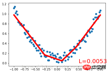
First Create a set of noisy quadratic functions to fit the data and place them in Variable. Define a class Net for building neural networks, inheriting the torch.nn.Module class. The parameters of the number of input neurons, hidden layer neurons, and output neurons are defined in the construction method of the Net class. The construction method of the Net parent class is obtained through the super() method, and the structural form of each layer of the Net is defined in the form of attributes; definition Net's forward() method builds the neurons of each layer into a complete neural network forward path.

After defining the Net class, define a neural network instance. The Net class instance can directly print out the structural information of the neural network. Then define the optimizer and loss function of the neural network. Once these are defined, training can begin. optimizer.zero_grad(), loss.backward(), and optimizer.step() respectively clear the update parameter value of the previous step, perform backpropagation of the error and calculate the new update parameter value, and assign the calculated update value to the net .parameters(). Loop iterative training process.

Run result:

Net (

(hidden): Linear (1 -> 10)

 (predict): Linear (10 -> 1)

)

三、PyTorch实现简单分类

完整代码：

import torch 
from torch.autograd import Variable 
import torch.nn.functional as F 
import matplotlib.pyplot as plt 
 
# 生成数据 
# 分别生成2组各100个数据点，增加正态噪声，后标记以y0=0 y1=1两类标签，最后cat连接到一起 
n_data = torch.ones(100,2) 
# torch.normal(means, std=1.0, out=None) 
x0 = torch.normal(2*n_data, 1) # 以tensor的形式给出输出tensor各元素的均值，共享标准差 
y0 = torch.zeros(100) 
x1 = torch.normal(-2*n_data, 1) 
y1 = torch.ones(100) 
 
x = torch.cat((x0, x1), 0).type(torch.FloatTensor) # 组装（连接） 
y = torch.cat((y0, y1), 0).type(torch.LongTensor) 
 
# 置入Variable中 
x, y = Variable(x), Variable(y) 
 
class Net(torch.nn.Module): 
  def __init__(self, n_feature, n_hidden, n_output): 
    super(Net, self).__init__() 
    self.hidden = torch.nn.Linear(n_feature, n_hidden) 
    self.out = torch.nn.Linear(n_hidden, n_output) 
 
  def forward(self, x): 
    x = F.relu(self.hidden(x)) 
    x = self.out(x) 
    return x 
 
net = Net(n_feature=2, n_hidden=10, n_output=2) 
print(net) 
 
optimizer = torch.optim.SGD(net.parameters(), lr=0.012) 
loss_func = torch.nn.CrossEntropyLoss() 
 
plt.ion() 
plt.show() 
 
for t in range(100): 
  out = net(x) 
  loss = loss_func(out, y) # loss是定义为神经网络的输出与样本标签y的差别，故取softmax前的值 
 
  optimizer.zero_grad() 
  loss.backward() 
  optimizer.step() 
 
  if t % 2 == 0: 
    plt.cla() 
    # 过了一道 softmax 的激励函数后的最大概率才是预测值 
    # torch.max既返回某个维度上的最大值，同时返回该最大值的索引值 
    prediction = torch.max(F.softmax(out), 1)[1] # 在第1维度取最大值并返回索引值 
    pred_y = prediction.data.numpy().squeeze() 
    target_y = y.data.numpy() 
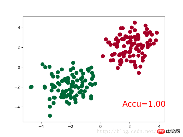
    plt.scatter(x.data.numpy()[:, 0], x.data.numpy()[:, 1], c=pred_y, s=100, lw=0, cmap='RdYlGn') 
    accuracy = sum(pred_y == target_y)/200 # 预测中有多少和真实值一样 
    plt.text(1.5, -4, 'Accu=%.2f' % accuracy, fontdict={'size': 20, 'color': 'red'}) 
    plt.pause(0.1) 
 
plt.ioff() 
plt.show()

神经网络结构部分的Net类与前文的回归部分的结构相同。

需要注意的是，在循环迭代训练部分，out定义为神经网络的输出结果，计算误差loss时不是使用one-hot形式的，loss是定义在out与y上的torch.nn.CrossEntropyLoss()，而预测值prediction定义为out经过Softmax后（将结果转化为概率值）的结果。

运行结果：

Net (

 (hidden): Linear (2 -> 10)

  (out):Linear (10 -> 2)

)

四、补充知识

1. super()函数

在定义Net类的构造方法的时候，使用了super(Net,self).__init__()语句，当前的类和对象作为super函数的参数使用，这条语句的功能是使Net类的构造方法获得其超类（父类）的构造方法，不影响对Net类单独定义构造方法，且不必关注Net类的父类到底是什么，若需要修改Net类的父类时只需修改class语句中的内容即可。

2. torch.normal()

torch.normal()可分为三种情况：（1）torch.normal(means,std, out=None)中means和std都是Tensor，两者的形状可以不必相同，但Tensor内的元素数量必须相同，一一对应的元素作为输出的各元素的均值和标准差；（2）torch.normal(mean=0.0, std, out=None)中mean是一个可定义的float，各个元素共享该均值；（3）torch.normal(means,std=1.0, out=None)中std是一个可定义的float，各个元素共享该标准差。

3. torch.cat(seq, dim=0)

torch.cat可以将若干个Tensor组装连接起来，dim指定在哪个维度上进行组装。

4. torch.max()

（1）torch.max(input)→ float

input是tensor，返回input中的最大值float。

（2）torch.max(input,dim, keepdim=True, max=None, max_indices=None) -> (Tensor, LongTensor)

同时返回指定维度=dim上的最大值和该最大值在该维度上的索引值。

相关推荐：

PyTorch快速搭建神经网络及其保存提取方法详解

PyTorch上实现卷积神经网络CNN的方法

The above is the detailed content of Example of building a simple neural network on PyTorch to implement regression and classification. For more information, please follow other related articles on the PHP Chinese website!