
Home > Article > Backend Development > How TensorFlow implements random training and batch training

This article mainly introduces the method of TensorFlow to implement random training and batch training. Now I will share it with you and give you a reference. Let’s take a look together
TensorFlow updates model variables. It can operate on one data point at a time or on large amounts of data at once. Operating on a single training example can lead to a "quirky" learning process, but training with large batches can be computationally expensive. Which type of training is chosen is very critical to the convergence of the machine learning algorithm.
In order for TensorFlow to calculate variable gradients for backpropagation to work, we must measure the loss on one or more samples.
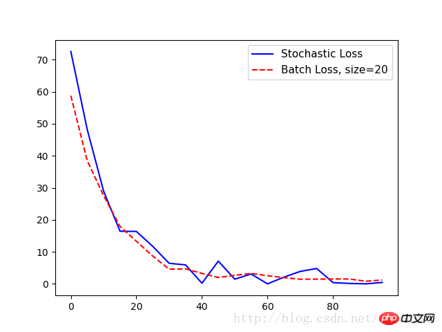
Random training will randomly sample pairs of training data and target data to complete the training. Another option is to average the loss for gradient calculation in a large batch training, and the batch training size can be expanded to the entire data set at once. Here we show how to extend the previous example of a regression algorithm - using random training and batch training.
Batch training and random training differ in their optimizer methods and convergence.
# 随机训练和批量训练
#----------------------------------
#
# This python function illustrates two different training methods:
# batch and stochastic training. For each model, we will use
# a regression model that predicts one model variable.
import matplotlib.pyplot as plt
import numpy as np
import tensorflow as tf
from tensorflow.python.framework import ops
ops.reset_default_graph()
# 随机训练:
# Create graph
sess = tf.Session()
# 声明数据
x_vals = np.random.normal(1, 0.1, 100)
y_vals = np.repeat(10., 100)
x_data = tf.placeholder(shape=[1], dtype=tf.float32)
y_target = tf.placeholder(shape=[1], dtype=tf.float32)
# 声明变量 (one model parameter = A)
A = tf.Variable(tf.random_normal(shape=[1]))
# 增加操作到图
my_output = tf.multiply(x_data, A)
# 增加L2损失函数
loss = tf.square(my_output - y_target)
# 初始化变量
init = tf.global_variables_initializer()
sess.run(init)
# 声明优化器
my_opt = tf.train.GradientDescentOptimizer(0.02)
train_step = my_opt.minimize(loss)
loss_stochastic = []
# 运行迭代
for i in range(100):
 rand_index = np.random.choice(100)
 rand_x = [x_vals[rand_index]]
 rand_y = [y_vals[rand_index]]
 sess.run(train_step, feed_dict={x_data: rand_x, y_target: rand_y})
 if (i+1)%5==0:
  print('Step #' + str(i+1) + ' A = ' + str(sess.run(A)))
  temp_loss = sess.run(loss, feed_dict={x_data: rand_x, y_target: rand_y})
  print('Loss = ' + str(temp_loss))
  loss_stochastic.append(temp_loss)
# 批量训练:
# 重置计算图
ops.reset_default_graph()
sess = tf.Session()

# 声明批量大小
# 批量大小是指通过计算图一次传入多少训练数据
batch_size = 20

# 声明模型的数据、占位符
x_vals = np.random.normal(1, 0.1, 100)
y_vals = np.repeat(10., 100)
x_data = tf.placeholder(shape=[None, 1], dtype=tf.float32)
y_target = tf.placeholder(shape=[None, 1], dtype=tf.float32)

# 声明变量 (one model parameter = A)
A = tf.Variable(tf.random_normal(shape=[1,1]))

# 增加矩阵乘法操作(矩阵乘法不满足交换律)
my_output = tf.matmul(x_data, A)

# 增加损失函数
# 批量训练时损失函数是每个数据点L2损失的平均值
loss = tf.reduce_mean(tf.square(my_output - y_target))

# 初始化变量
init = tf.global_variables_initializer()
sess.run(init)

# 声明优化器
my_opt = tf.train.GradientDescentOptimizer(0.02)
train_step = my_opt.minimize(loss)

loss_batch = []
# 运行迭代
for i in range(100):
 rand_index = np.random.choice(100, size=batch_size)
 rand_x = np.transpose([x_vals[rand_index]])
 rand_y = np.transpose([y_vals[rand_index]])
 sess.run(train_step, feed_dict={x_data: rand_x, y_target: rand_y})
 if (i+1)%5==0:
  print('Step #' + str(i+1) + ' A = ' + str(sess.run(A)))
  temp_loss = sess.run(loss, feed_dict={x_data: rand_x, y_target: rand_y})
  print('Loss = ' + str(temp_loss))
  loss_batch.append(temp_loss)

plt.plot(range(0, 100, 5), loss_stochastic, 'b-', label='Stochastic Loss')
plt.plot(range(0, 100, 5), loss_batch, 'r--', label='Batch Loss, size=20')
plt.legend(loc='upper right', prop={'size': 11})
plt.show()
Output:
Step #5 A = [ 1.47604525]
Loss = [ 72.55678558]
Step #10 A = [ 3.01128507]
Loss = [ 48.22986221]
Step #15 A = [ 4.27042341]
Loss = [ 28.97912598]
Step #20 A = [ 5.2984333]
Loss = [ 16.44779968]
Step #25 A = [ 6.17473984]
Loss = [ 16.373312]
Step #30 A = [ 6.89866304]
Loss = [ 11.71054649]
Step #35 A = [ 7.39849901]
Loss = [ 6.42773056]
Step #40 A = [ 7.84618378]
Loss = [ 5.92940331]
Step #45 A = [ 8.15709782]
Loss = [ 0.2142024]
Step #50 A = [ 8.54818344]
Loss = [ 7.11651039]
Step #55 A = [ 8.82354641]
Loss = [ 1.47823763]
Step #60 A = [ 9.07896614]
Loss = [ 3.08244276]
Step #65 A = [ 9.24868107]
Loss = [ 0.01143846]
Step #70 A = [ 9.36772251]
Loss = [ 2.10078788]
Step #75 A = [ 9.49171734]
Loss = [ 3.90913701]
Step #80 A = [ 9.6622715]
Loss = [ 4.80727625]
Step #85 A = [ 9.73786926]
Loss = [ 0.39915398]
Step #90 A = [ 9.81853104]
Loss = [ 0.14876099]
Step #95 A = [ 9.90371323]
Loss = [ 0.01657014]
Step #100 A = [ 9.86669159]
Loss = [0.444787]
Step #5 A = [[ 2.34371352]]
Loss = 58.766
Step #10 A = [[ 3.74766445]]
Loss = 38.4875
Step # 15 A = [[ 4.88928795]]
Loss = 27.5632
Step #20 A = [[ 5.82038736]]
Loss = 17.9523
Step #25 A = [[ 6.58999157]]
Loss = 13.3245
Step #30 A = [[ 7.20851326]]
Loss = 8.68099
Step #35 A = [[ 7.71694899]]
Loss = 4.60659
Step #40 A = [[ 8.1296711]]
Loss = 4.70107
Step #45 A = [[ 8.47107315]]
Loss = 3.28318
Step #50 A = [[ 8.74283409]]
Loss = 1.99057
Step #55 A = [[ 8.98811722]]
Loss = 2.66906
Step #60 A = [[ 9.18062305]]
Loss = 3.26207
Step #65 A = [[ 9.31655025]]
Loss = 2.55459
Step #70 A = [[ 9.43130589]]
Loss = 1.95839
Step #75 A = [[ 9.55670166]]
Loss = 1.46504
Step #80 A = [[ 9.6354847]]
Loss = 1.49021
Step #85 A = [[ 9.73470974]]
Loss = 1.53289
Step #90 A = [[ 9.77956581]]
Loss = 1.52173
Step #95 A = [[ 9.83666706]]
Loss = 0.819207
Step #100 A = [[ 9.85569191]]
Loss = 1.2197
| Advantages | Disadvantages | |
|---|---|---|
| Out of local minimum | Generally more iterations are needed to converge | |
| Get the minimum loss quickly | Consume more computing resources |
A brief discussion on tensorflow1.0 pooling layer (pooling) and fully connected layer (dense)
A brief discussion on saving and restoring the Tensorflow model
The above is the detailed content of How TensorFlow implements random training and batch training. For more information, please follow other related articles on the PHP Chinese website!