Detailed explanation of using least squares method in Python

The reason why I say "use" rather than "implement" is because python's related class libraries have already helped us implement specific algorithms, and we only need to learn to use them. With the gradual mastery and accumulation of technology, when the algorithms in the class library can no longer meet our own needs, we can also try to implement various algorithms in our own way.

Let’s get back to the subject, what is the “least squares method”?

Definition: The least squares method (also known as the least squares method) is a mathematical optimization technique that finds the best function matching of the data by minimizing the sum of squares of the errors.

Function: The least squares method can be used to easily obtain unknown data, and minimize the sum of square errors between the obtained data and the actual data.

Principle: Determine the straight line position by "minimizing the sum of squares of the residuals" (in mathematical statistics, the residual refers to the difference between the actual observed value and the estimated value)

Basic idea: For Univariate linear regression model, assuming that n sets of observation values ​​(X1, Y1), (X2, Y2), ..., (Xn, Yn) are obtained from the population. For these n points in the plane, countless curves can be used to fitting. Linear regression requires the sample regression function to fit this set of values ​​as well as possible. In other words, this straight line should be as centered as possible in the sample data. Therefore, the criterion for selecting the best fitting curve can be determined as: minimizing the total fitting error (ie, the total residual error).

The implementation code is as follows, and the code has been commented in detail:

##最小二乘法
import numpy as np   ##科学计算库 
import scipy as sp   ##在numpy基础上实现的部分算法库
import matplotlib.pyplot as plt  ##绘图库
from scipy.optimize import leastsq  ##引入最小二乘法算法

'''
     设置样本数据，真实数据需要在这里处理
'''
##样本数据(Xi,Yi)，需要转换成数组(列表)形式
Xi=np.array([6.19,2.51,7.29,7.01,5.7,2.66,3.98,2.5,9.1,4.2])
Yi=np.array([5.25,2.83,6.41,6.71,5.1,4.23,5.05,1.98,10.5,6.3])

'''
    设定拟合函数和偏差函数
    函数的形状确定过程：
    1.先画样本图像
    2.根据样本图像大致形状确定函数形式(直线、抛物线、正弦余弦等)
'''

##需要拟合的函数func :指定函数的形状
def func(p,x):
    k,b=p
    return k*x+b

##偏差函数：x,y都是列表:这里的x,y更上面的Xi,Yi中是一一对应的
def error(p,x,y):
    return func(p,x)-y

'''
    主要部分：附带部分说明
    1.leastsq函数的返回值tuple，第一个元素是求解结果，第二个是求解的代价值(个人理解)
    2.官网的原话（第二个值）：Value of the cost function at the solution
    3.实例：Para=>(array([ 0.61349535,  1.79409255]), 3)
    4.返回值元组中第一个值的数量跟需要求解的参数的数量一致
'''

#k,b的初始值，可以任意设定,经过几次试验，发现p0的值会影响cost的值：Para[1]
p0=[1,20]

#把error函数中除了p0以外的参数打包到args中(使用要求)
Para=leastsq(error,p0,args=(Xi,Yi))

#读取结果
k,b=Para[0]
print("k=",k,"b=",b)
print("cost："+str(Para[1]))
print("求解的拟合直线为:")
print("y="+str(round(k,2))+"x+"+str(round(b,2)))

'''
   绘图，看拟合效果.
   matplotlib默认不支持中文，label设置中文的话需要另行设置
   如果报错，改成英文就可以
'''

#画样本点
plt.figure(figsize=(8,6)) ##指定图像比例： 8：6
plt.scatter(Xi,Yi,color="green",label="样本数据",linewidth=2) 

#画拟合直线
x=np.linspace(0,12,100) ##在0-15直接画100个连续点
y=k*x+b ##函数式
plt.plot(x,y,color="red",label="拟合直线",linewidth=2) 
plt.legend() #绘制图例
plt.show()

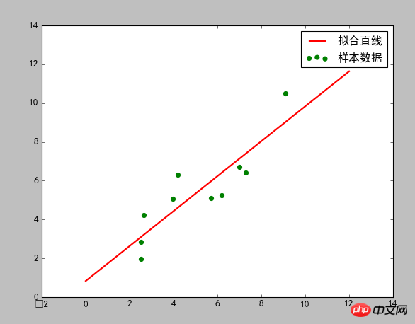
The result is as follows:

Output result:

k= 0.900458420439 b = 0.831055638877
cost: 1
The fitted straight line solved is:
y=0.9x+0.83

Drawing result:

The above is the detailed content of Detailed explanation of using least squares method in Python. For more information, please follow other related articles on the PHP Chinese website!