How to create gradient transparent color graphic method for Excel column chart

php Xiaobian Strawberry teaches you how to create gradient transparent color graphics and text in Excel column charts. During the production process of column charts in Excel, the transparency and color gradient can be adjusted to increase the beauty of the chart and the effect of information transmission. In this article, we will introduce in detail how to achieve the color gradient effect of column charts through simple operations, making your Excel charts more attractive and readable.

1. Open the chart. The system default is opaque.

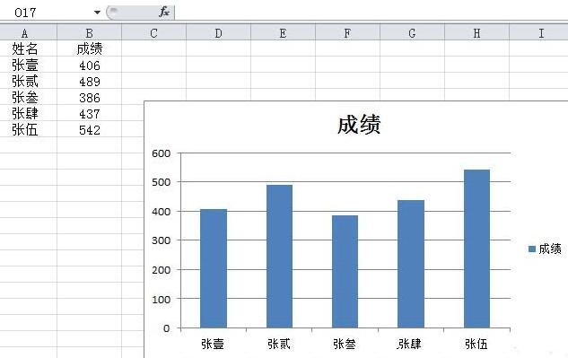
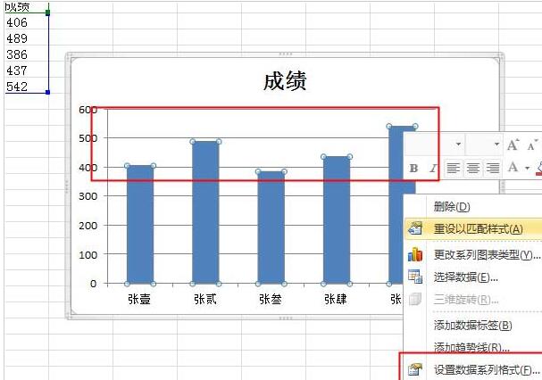
2. Select all data series, right-click on the data series, and click Format Data Series.

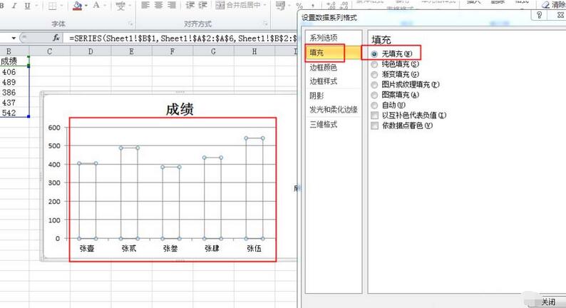
3. A dialog box pops up, click Fill, and select No Fill. Looking at the chart, there is now only an outline of the figure. In this case, you can choose no fill.

4. If you still want a little color, click on the solid color fill. There is a transparency setting below.

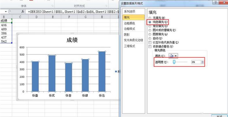
5. Pull the pull bar on the right side of the transparency or directly enter the transparency value in the back column to see that the chart is transparent.

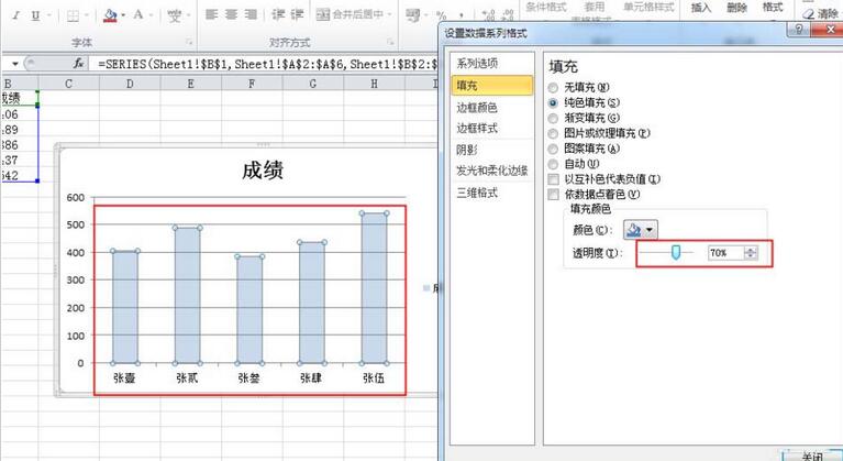
6. You can also click Gradient Fill. There are also transparency settings below.

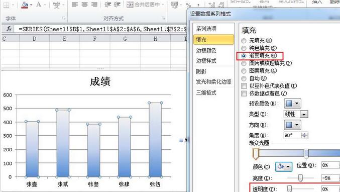
7. Pull the slider on the right side of the transparency or enter the transparency value directly in the back column. You will see that this time only the lighter color becomes transparent, while the darker color becomes transparent. no change.

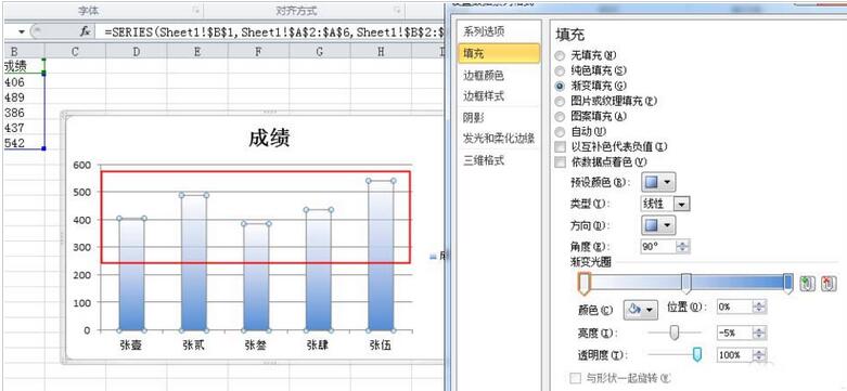
The above is the detailed content of How to create gradient transparent color graphic method for Excel column chart. For more information, please follow other related articles on the PHP Chinese website!