This article brings you relevant knowledge about excel, which mainly organizes issues related to the application of super tables, including table creation, summary, dynamic range, etc. Let’s talk about it together Take a look, hope it helps everyone.

Related learning recommendations: excel tutorial
There are three "fennel" in fennel beans Similarly, there are several different ways to create tables.
The first method:
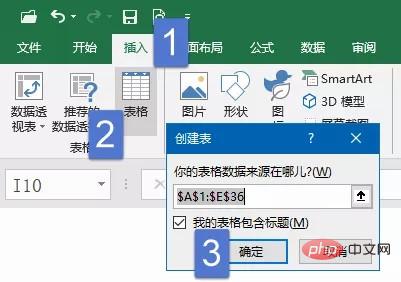
Click any cell in the data area and click the [Table] button under the [Insert] tab. At this time, Excel will automatically help us select the adjacent area. , click [OK] in the dialog box, OK.
Second method:
Click any cell in the data area, hold down the Ctrl key, and then press T, or hold down Ctrl If you hold down the key and press L again, the [Create Table] dialog box will pop up.
The third method:
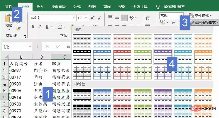
Click any cell in the data area, [Start] → [Apply Table Format], a bunch of built-in Style, just click one of them to bring up the [Create Table] dialog box.
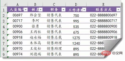
After converting to [Table], the table style will be automatically applied to the data table, just like the preview effect we just saw in the picture above.
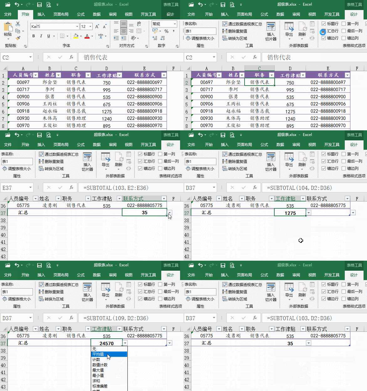
Click any area of the "Table" and select "Summary Row" under the [Design] tab. Wonderful What happened:
A "Summary" row will automatically appear in the last row of the "Table". Click any cell in this row to select the summary method in the drop-down menu.
After adding [Summary Row], what should I do if I want to add a few records?
Click the rightmost cell of the previous row of the summary row and press the Tab key.
The table will automatically expand the range, and the summary row will automatically move down.
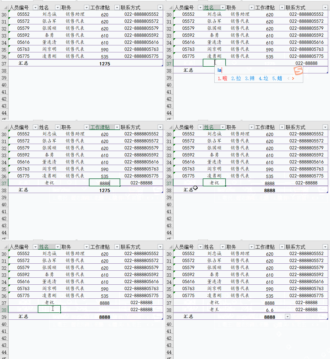
Using this feature, after inserting the table and then inserting the pivot table, you can solve the problem of automatic expansion of the data source of the pivot table.
If a column range in the "table" is referenced in the formula and the data in the "table" increases, the formula reference range will also be automatically expanded.
After inserting the "table", a small triangle button will be automatically added to the lower right corner of the cell in the first row of the table. This small triangle button is What is it? Just filter it, remove the unnecessary ones, and keep only the necessary ones.
After filtering in "Table", the summary formula of the last row can be automatically updated. Whatever you need, Excel will summarize it.
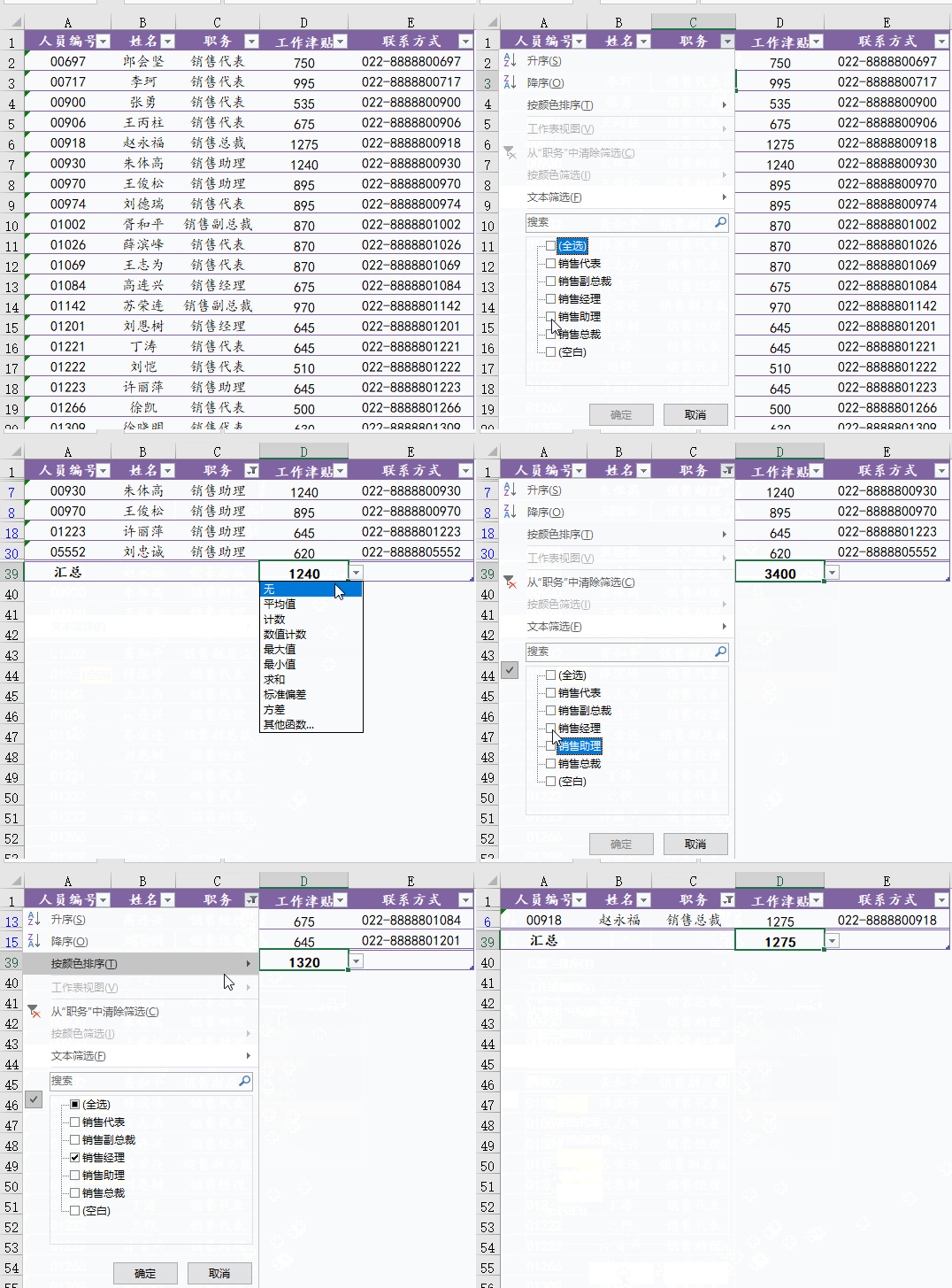
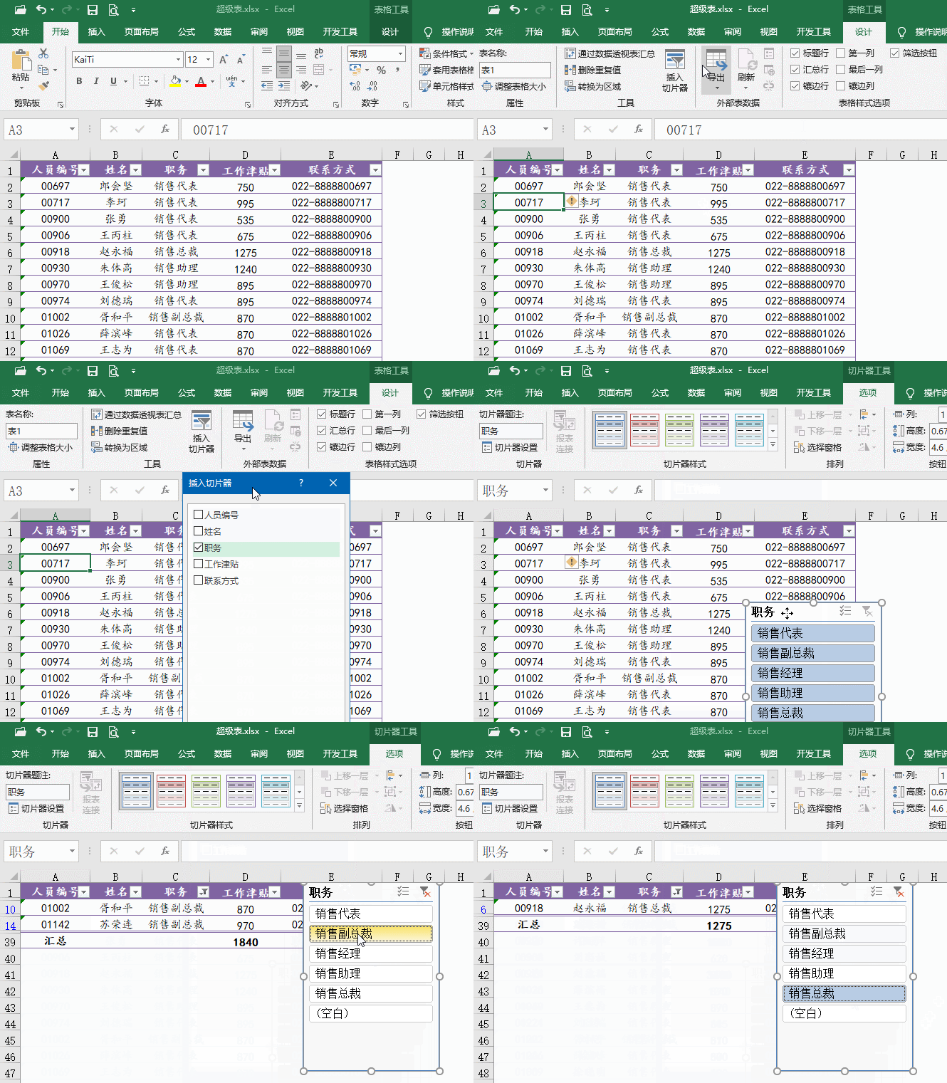
To say that there are 666 filtering operations above, there are 777 operations next. Insert a slicer to make sifting easier.
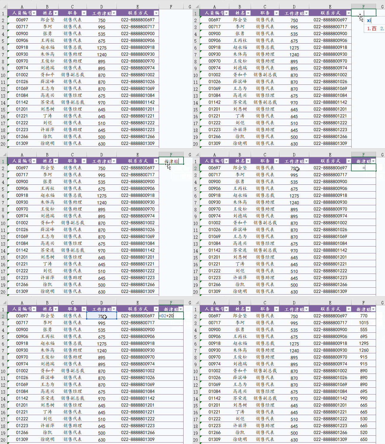
Enter the formulas in the "Table". Just press Enter and these formulas will be automatically filled to the end of the table. One line, one word: so fast!
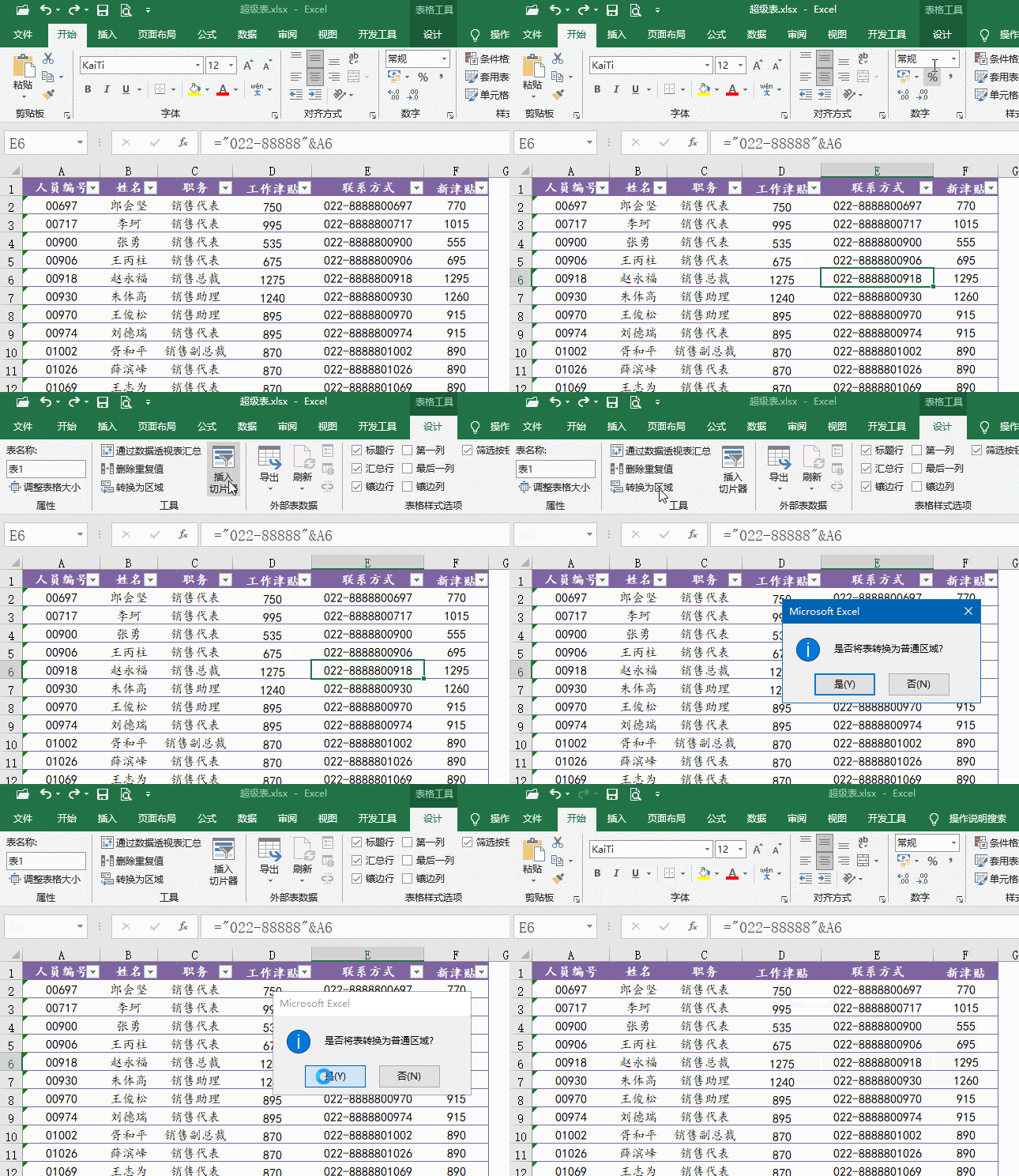
If one day, we no longer need to use the "table" function, how can we turn it into a regular table?
Click any cell in the [Table] area, and then select [Convert to Range] under the [Design] tab.
The data is still the data, but the "table" is no longer that "table".
Related learning recommendations: excel tutorial
The above is the detailed content of Summarize the application of Excel super table. For more information, please follow other related articles on the PHP Chinese website!