If you want to know more about excel, you can click:Excel Tutorial
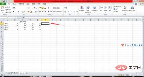
## 1. First, open the Excel table you want to use. I used student monthly exam score trend analysis as an example to create sparklines. As shown in the figure, open the data table.

2. Next, position a cell to make it the active cell. In this example, we click on cell F2, then this cell is the cell where we want to insert the sparkline.

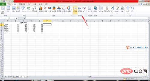
3. Then, use the left mouse button to click the sparkline type you want to select in the "Sparklines" group on the "Insert" tab. In this example, we're selecting a line chart, so click on the line chart icon.

4. After clicking the line chart chart, a dialog box will pop up. In the "Data Range" of the dialog box, enter the range of the data you want to create the sparkline for, or directly drag the selection area with the mouse on the cell.

5. Click OK, and the mini-graph will be generated.

# 6. Use the fill handle to quickly generate the mini-map below. We are done creating the sparkline.

The above is the detailed content of How to create mini charts in Excel in 2007. For more information, please follow other related articles on the PHP Chinese website!
Statement:
The content of this article is voluntarily contributed by netizens, and the copyright belongs to the original author. This site does not assume corresponding legal responsibility. If you find any content suspected of plagiarism or infringement, please contact admin@php.cn


