최단 경로 찾기

두 정점 사이의 최단 경로는 총 가중치가 최소인 경로입니다.
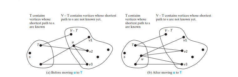
모서리에 음수가 아닌 가중치가 있는 그래프가 주어지면 네덜란드 컴퓨터 과학자인 Edsger Dijkstra가 두 정점 사이의 최단 경로를 찾는 잘 알려진 알고리즘을 발견했습니다. 정점 s에서 정점 v까지의 최단 경로를 찾기 위해 Dijkstra의 알고리즘은 s에서 모든 정점까지의 최단 경로를 찾습니다. 그래서 Dijkstra의 알고리즘은 단일 소스 최단 경로 알고리즘으로 알려져 있습니다. 알고리즘은 cost[v]를 사용하여 정점 v에서 소스 정점 s까지의 최단 경로 비용을 저장합니다. 비용은 0입니다. 처음에는 다른 모든 정점에 대해 cost[v]에 무한대를 할당합니다. 알고리즘은 V – T에서 cost[u]가 가장 작은 정점 u를 반복적으로 찾아 u를 T로 이동합니다. .

알고리즘은 아래 코드에 설명되어 있습니다.

Input: a graph G = (V, E) with non-negative weights
Output: a shortest path tree with the source vertex s as the root
 1 ShortestPathTree getShortestPath(s) {
 2 Let T be a set that contains the vertices whose
 3 paths to s are known; Initially T is empty;
 4 Set cost[s] = 0; and cost[v] = infinity for all other vertices in V;
 5
 6 while (size of T < n) {
 7 Find u not in T with the smallest cost[u];
 8 Add u to T;
 9 for (each v not in T and (u, v) in E)
10 if (cost[v] > cost[u] + w(u, v)) {
11 cost[v] = cost[u] + w(u, v); parent[v] = u;
12 }
13 }
14 }

이 알고리즘은 최소 스패닝 트리를 찾는 Prim의 알고리즘과 매우 유사합니다. 두 알고리즘 모두 정점을 T 및 V - T의 두 세트로 나눕니다. Prim의 알고리즘의 경우 T 세트에는 이미 트리에 추가된 정점이 포함됩니다. Dijkstra의 경우 세트 T에는 소스까지의 최단 경로가 발견된 정점이 포함됩니다. 두 알고리즘 모두 V – T에서 정점을 반복적으로 찾아 T에 추가합니다. Prim 알고리즘의 경우 정점은 가장자리의 가중치가 최소인 집합의 일부 정점과 인접해 있습니다. Dijkstra 알고리즘에서 정점은 소스에 대한 총 비용이 최소인 집합의 일부 정점과 인접해 있습니다.

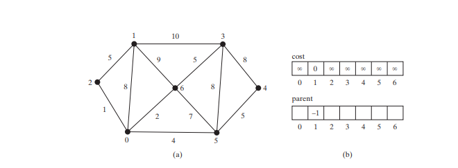
알고리즘은 cost[s]를 0(4번째 줄)으로 설정하고 다른 모든 정점에 대해 cost[v]를 무한대로 설정하는 것으로 시작합니다. 그런 다음 V – T의 정점(예: u)을 비용[u]이 가장 작은 T에 계속해서 추가합니다(7행 – 8) 아래 그림과 같이 a. T에 u를 추가한 후 알고리즘은 각 vcost[v] 및 parent[v]를 업데이트합니다. > T에 없음 (u, v)가 T에 있고 cost[v] > 비용[u] + w(u, v) (라인 10–11).

1이라고 가정합니다. 따라서 아래 그림 b에 표시된 것처럼 cost[1] = 0이고 다른 모든 꼭짓점의 비용은 초기에 입니다. parent[i]를 사용하여 경로에서 i의 부모를 나타냅니다. 편의상 소스 노드의 상위 노드를 -1으로 설정합니다.

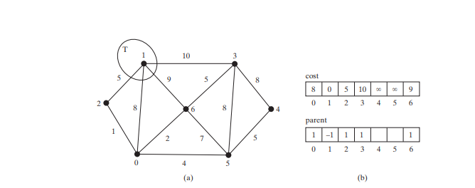
T는 비어 있습니다. 알고리즘은 비용이 가장 작은 정점을 선택합니다. 이 경우 정점은 1입니다. 알고리즘은 아래 그림과 같이 T에 1을 추가합니다. 이후 1에 인접한 각 정점의 비용을 조정합니다. 이제 아래 그림 b와 같이 꼭지점 2, 0, 6, 3과 해당 부모의 비용이 업데이트됩니다.

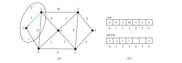
2, 0, 6, 3은 원본 정점에 인접하고 정점 2는 V-T에서 비용이 가장 작은 항목이므로 아래 그림과 같이 T에 2를 추가하고 정점의 비용과 부모를 업데이트합니다. V-T이고 2에 인접합니다. cost[0]는 이제 6으로 업데이트되고 해당 상위 항목은 2로 설정됩니다. 1에서 2까지의 화살표 선은 2가 추가된 후 1이 2의 상위임을 나타냅니다. ㅇ.

이제 T에는 {1, 2}이 포함됩니다. Vertex 0은 V-T에서 cost가 가장 작은 Vertex 0이므로 아래 그림과 같이 T에 0을 추가하고 V-T에 있고 해당하는 경우 0에 인접한 정점에 대한 비용 및 부모입니다. cost[5]는 이제 10으로 업데이트되고 상위 항목은 0으로 설정되며 cost[6]은 이제 cost[6]으로 업데이트됩니다. 🎜>8

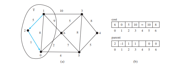0으로 설정됩니다.

이제 T에는 {1, 2, 0}이 포함됩니다. Vertex 6은 V-T에서 cost가 가장 작은 Vertex 6이므로 아래 그림과 같이 T에 6

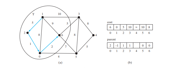V-T에 있고 해당하는 경우

에 인접한 정점에 대한 비용 및 부모입니다. 이제 T에는 {1, 2, 0, 6}이 포함됩니다. Vertex 3 또는 5는 V-T에서 비용이 가장 작은 것입니다. T에 3 또는 5을 추가할 수 있습니다. 아래 그림과 같이 T에 3을 추가하고 V-T에 있고 3에 인접한 정점에 대한 비용과 부모를 업데이트하겠습니다. 해당되는 경우. cost[4]

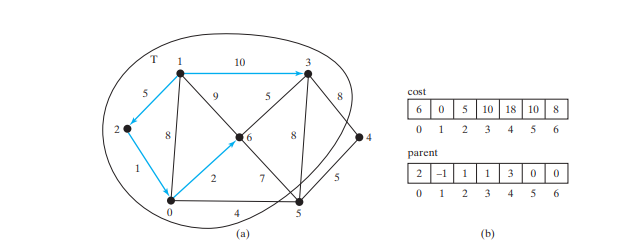18으로 업데이트되고 해당 상위 항목은

으로 설정됩니다. 현재 T에는 {1, 2, 0, 6, 3}. Vertex 5는 V-T에서 cost가 가장 작은 Vertex 5이므로 아래 그림과 같이 T에 5를 추가하고 V-T에 있고 해당하는 경우 5에 인접한 정점에 대한 비용 및 부모입니다.

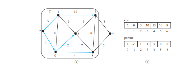는 이제 10

5으로 설정됩니다. 현재 T에는 {1, 2, 0, 6, 3, 5}. Vertex 4는 V-T

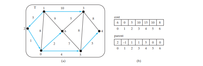4이므로 아래 그림과 같이

에 4를 추가합니다. 보시다시피 이 알고리즘은 본질적으로 소스 꼭짓점에서 모든 최단 경로를 찾아 소스 꼭짓점에 뿌리를 둔 트리를 생성합니다. 우리는 이 트리를 단일 소스 모든 최단 경로 트리(또는 간단히 최단 경로 트리)라고 부릅니다. 이 트리를 모델링하려면 아래 그림과 같이 Tree

ShortestPathTree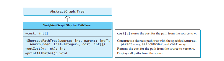라는 클래스를 정의하세요.

는 WeightedGraph.java의 200~224행에 있는 WeightedGraph의 내부 클래스로 정의됩니다. getShortestPath(int sourceVertex) 메소드는 WeightedGraph.java의 156~197행에서 구현되었습니다. 이 메서드는 cost[sourceVertex]를 0(162행)으로 설정하고 다른 모든 정점(159~161행)에 대해 cost[v]를 무한대로 설정합니다. sourceVertex의 부모는 -1

T는 최단 경로 트리(169행)에 추가된 정점을 저장하는 목록입니다. T에 추가되는 정점의 순서를 기록하기 위해 세트가 아닌 T

1. Find the vertex u with the smallest cost[u] (lines 175–181) and add it into T (line 183).
2. After adding u in T, update cost[v] and parent[v] for each v adjacent to u in V-T if cost[v] > cost[u] + w(u, v) (lines 186–192).

Once all vertices from s are added to T, an instance of ShortestPathTree is created (line 196).

The ShortestPathTree class extends the Tree class (line 200). To create an instance of ShortestPathTree, pass sourceVertex, parent, T, and cost (lines 204–205). sourceVertex becomes the root in the tree. The data fields root, parent, and searchOrder are defined in the Tree class, which is an inner class defined in AbstractGraph.

Note that testing whether a vertex i is in T by invoking T.contains(i) takes O(n) time, since T is a list. Therefore, the overall time complexity for this implemention is O(n^3).

Dijkstra’s algorithm is a combination of a greedy algorithm and dynamic programming. It is a greedy algorithm in the sense that it always adds a new vertex that has the shortest distance to the source. It stores the shortest distance of each known vertex to the source and uses it later to avoid redundant computing, so Dijkstra’s algorithm also uses dynamic programming.

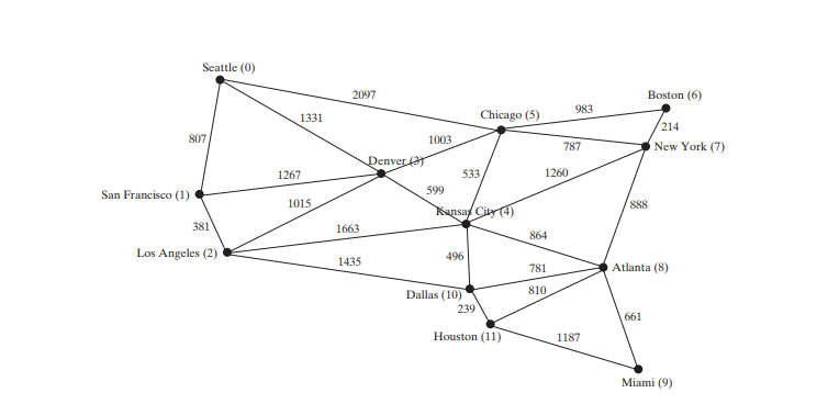
The code below gives a test program that displays the shortest paths from Chicago to all other cities in Figure below and the shortest paths from vertex 3 to all vertices for the graph in Figure below a, respectively.

package demo;

public class TestShortestPath {

    public static void main(String[] args) {
String[] vertices = {"Seattle", "San Francisco", "Los Angeles", "Denver", "Kansas City", "Chicago", "Boston", "New York", "Atlanta", "Miami", "Dallas", "Houston"};

        int[][] edges = {
                {0, 1, 807}, {0, 3, 1331}, {0, 5, 2097},
                {1, 0, 807}, {1, 2, 381}, {1, 3, 1267},
                {2, 1, 381}, {2, 3, 1015}, {2, 4, 1663}, {2, 10, 1435},
                {3, 0, 1331}, {3, 1, 1267}, {3, 2, 1015}, {3, 4, 599}, {3, 5, 1003},
                {4, 2, 1663}, {4, 3, 599}, {4, 5, 533}, {4, 7, 1260}, {4, 8, 864}, {4, 10, 496},
                {5, 0, 2097}, {5, 3, 1003}, {5, 4, 533}, {5, 6, 983}, {5, 7, 787},
                {6, 5, 983}, {6, 7, 214},
                {7, 4, 1260}, {7, 5, 787}, {7, 6, 214}, {7, 8, 888},
                {8, 4, 864}, {8, 7, 888}, {8, 9, 661}, {8, 10, 781}, {8, 11, 810},
                {9, 8, 661}, {9, 11, 1187},
                {10, 2, 1435}, {10, 4, 496}, {10, 8, 781}, {10, 11, 239},
                {11, 8, 810}, {11, 9, 1187}, {11, 10, 239}
        };

        WeightedGraph<String> graph1 = new WeightedGraph<>(vertices, edges);
        WeightedGraph<String>.ShortestPathTree tree1 = graph1.getShortestPath(graph1.getIndex("Chicago"));
        tree1.printAllPaths();

        // Display shortest paths from Houston to Chicago       
        System.out.println("Shortest path from Houston to Chicago: ");
        java.util.List<String> path = tree1.getPath(graph1.getIndex("Houston"));
        for(String s: path) {
            System.out.print(s + " ");
        }

        edges = new int[][]{
            {0, 1, 2}, {0, 3, 8},
            {1, 0, 2}, {1, 2, 7}, {1, 3, 3},
            {2, 1, 7}, {2, 3, 4}, {2, 4, 5},
            {3, 0, 8}, {3, 1, 3}, {3, 2, 4}, {3, 4, 6},
            {4, 2, 5}, {4, 3, 6}
        };

        WeightedGraph<Integer> graph2 = new WeightedGraph<>(edges, 5);
        WeightedGraph<Integer>.ShortestPathTree tree2 = graph2.getShortestPath(3);
        System.out.println("\n");
        tree2.printAllPaths();
    }

}

All shortest paths from Chicago are:
A path from Chicago to Seattle: Chicago Seattle (cost: 2097.0)
A path from Chicago to San Francisco:
Chicago Denver San Francisco (cost: 2270.0)
A path from Chicago to Los Angeles:
Chicago Denver Los Angeles (cost: 2018.0)
A path from Chicago to Denver: Chicago Denver (cost: 1003.0)
A path from Chicago to Kansas City: Chicago Kansas City (cost: 533.0)
A path from Chicago to Chicago: Chicago (cost: 0.0)
A path from Chicago to Boston: Chicago Boston (cost: 983.0)
A path from Chicago to New York: Chicago New York (cost: 787.0)
A path from Chicago to Atlanta:
Chicago Kansas City Atlanta (cost: 1397.0)
A path from Chicago to Miami:
Chicago Kansas City Atlanta Miami (cost: 2058.0)
A path from Chicago to Dallas: Chicago Kansas City Dallas (cost: 1029.0)
A path from Chicago to Houston:
Chicago Kansas City Dallas Houston (cost: 1268.0)
Shortest path from Houston to Chicago:
Houston Dallas Kansas City Chicago

All shortest paths from 3 are:
A path from 3 to 0: 3 1 0 (cost: 5.0)
A path from 3 to 1: 3 1 (cost: 3.0)
A path from 3 to 2: 3 2 (cost: 4.0)
A path from 3 to 3: 3 (cost: 0.0)
A path from 3 to 4: 3 4 (cost: 6.0)

The program creates a weighted graph for Figure above in line 27. It then invokes the getShortestPath(graph1.getIndex("Chicago")) method to return a Path object that contains all shortest paths from Chicago. Invoking printAllPaths() on the ShortestPathTree object displays all the paths (line 30).

The graphical illustration of all shortest paths from Chicago is shown in Figure below. The shortest paths from Chicago to the cities are found in this order: Kansas City, New York, Boston, Denver, Dallas, Houston, Atlanta, Los Angeles, Miami, Seattle, and San Francisco.

위 내용은 최단 경로 찾기의 상세 내용입니다. 자세한 내용은 PHP 중국어 웹사이트의 기타 관련 기사를 참조하세요!