


コンピュータービジョンにおける最も基本的な手順の 1 つである画像セグメンテーションにより、システムは画像内のさまざまな領域を分解して分析できます。物体認識、医療画像処理、自動運転のいずれを扱う場合でも、セグメンテーションは画像を意味のある部分に分割するものです。
このタスクでは深層学習モデルの人気が高まり続けていますが、デジタル画像処理における従来の技術は依然として強力で実用的です。この投稿でレビューされているアプローチには、しきい値処理、エッジ検出、領域ベース、および細胞画像解析用のよく知られたデータセットである MIVIA HEp-2 画像データセットを実装することによるクラスタリングが含まれます。
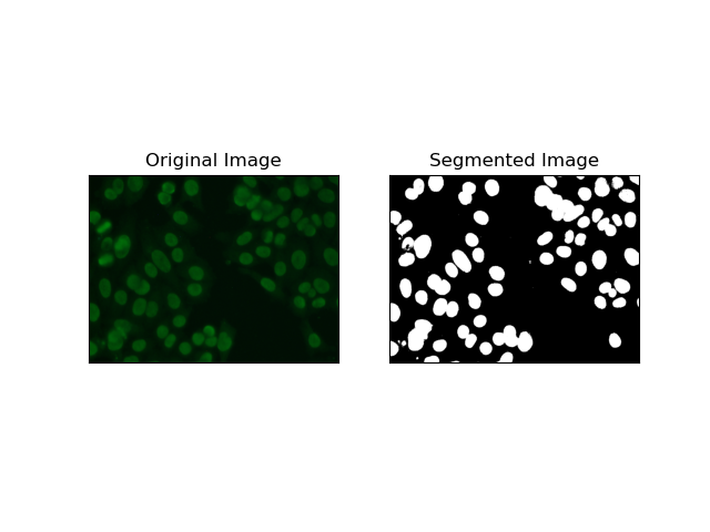
MIVIA HEp-2 画像データセットは、HEp-2 細胞による抗核抗体 (ANA) のパターンを分析するために使用される細胞の写真のセットです。これは、蛍光顕微鏡によって撮影された 2D 写真で構成されています。これにより、セグメンテーション タスク、特に細胞領域の検出が最も重要な医療画像分析に関係するタスクに非常に適しています。
ここで、これらの画像の処理に使用されるセグメンテーション手法に移り、F1 スコアに基づいてパフォーマンスを比較しましょう。
閾値処理は、ピクセル強度に基づいてグレースケール画像をバイナリ画像に変換するプロセスです。 MIVIA HEp-2 データセットでは、このプロセスはバックグラウンドからの細胞抽出に役立ちます。これは、最適なしきい値を自己計算するため、特に Otsu の方法 では、比較的大きなレベルまでシンプルかつ効果的です。
Otsu のメソッド は自動しきい値処理方法であり、クラス内分散を最小限に抑える最適なしきい値を見つけようとし、それによって前景 (セル) と背景の 2 つのクラスを分離します。このメソッドは画像のヒストグラムを検査し、各クラスのピクセル強度分散の合計が最小化される完全なしきい値を計算します。
# Thresholding Segmentation
def thresholding(img):
    # Convert image to grayscale
    gray = cv.cvtColor(img, cv.COLOR_BGR2GRAY)

    # Apply Otsu's thresholding
    _, thresh = cv.threshold(gray, 0, 255, cv.THRESH_BINARY + cv.THRESH_OTSU)

    return thresh
エッジ検出は、MIVIA HEp-2 データセット内のセル エッジなど、オブジェクトまたは領域の境界の識別に関係します。突然の強度変化を検出するために利用可能な多くの方法の中で、Canny Edge Detector が最良であり、したがって細胞境界の検出に使用するのに最も適した方法です。
Canny Edge Detector は、強度の強い勾配の領域を検出することでエッジを検出できる多段階アルゴリズムです。このプロセスには、ガウス フィルターによる平滑化、強度勾配の計算、スプリアス応答を除去するための非最大抑制の適用、および顕著なエッジのみを保持するための最終的な二重閾値処理が含まれます。
# Edge Detection Segmentation
def edge_detection(img):
    # Convert image to grayscale
    gray = cv.cvtColor(img, cv.COLOR_BGR2GRAY)

    # Apply Gaussian blur
    gray = cv.GaussianBlur(gray, (3, 3), 0)

    # Calculate lower and upper thresholds for Canny edge detection
    sigma = 0.33
    v = np.median(gray)
    lower = int(max(0, (1.0 - sigma) * v))
    upper = int(min(255, (1.0 + sigma) * v))

    # Apply Canny edge detection
    edges = cv.Canny(gray, lower, upper)

    # Dilate the edges to fill gaps
    kernel = np.ones((5, 5), np.uint8)
    dilated_edges = cv.dilate(edges, kernel, iterations=2)

    # Clean the edges using morphological opening
    cleaned_edges = cv.morphologyEx(dilated_edges, cv.MORPH_OPEN, kernel, iterations=1)

    # Find connected components and filter out small components
    num_labels, labels, stats, _ = cv.connectedComponentsWithStats(
        cleaned_edges, connectivity=8
    )
    min_size = 500
    filtered_mask = np.zeros_like(cleaned_edges)
    for i in range(1, num_labels):
        if stats[i, cv.CC_STAT_AREA] >= min_size:
            filtered_mask[labels == i] = 255

    # Find contours of the filtered mask
    contours, _ = cv.findContours(
        filtered_mask, cv.RETR_EXTERNAL, cv.CHAIN_APPROX_SIMPLE
    )

    # Create a filled mask using the contours
    filled_mask = np.zeros_like(gray)
    cv.drawContours(filled_mask, contours, -1, (255), thickness=cv.FILLED)

    # Perform morphological closing to fill holes
    final_filled_image = cv.morphologyEx(
        filled_mask, cv.MORPH_CLOSE, kernel, iterations=2
    )

    # Dilate the final filled image to smooth the edges
    final_filled_image = cv.dilate(final_filled_image, kernel, iterations=1)

    return final_filled_image

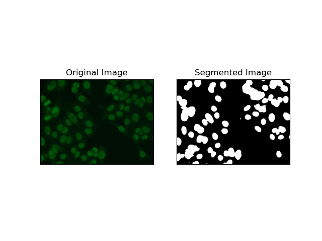
領域ベースのセグメンテーションは、強度や色などの特定の基準に応じて、類似したピクセルを領域にグループ化します。 ウォーターシェッドセグメンテーション 技術を使用すると、HEp-2 細胞画像をセグメント化し、細胞を表す領域を検出できるようになります。ピクセル強度を地形的な表面として考慮し、特徴的な領域の輪郭を描きます。
流域セグメンテーション は、ピクセルの強度を地形的な表面として扱います。このアルゴリズムは「盆地」を特定し、その中で極小値を特定し、これらの盆地を徐々に浸水させて個別の領域を拡大します。この技術は、顕微鏡画像内の細胞の場合のように、接触しているオブジェクトを分離したい場合に非常に役立ちますが、ノイズに敏感になる可能性があります。プロセスはマーカーによってガイドでき、多くの場合、過剰なセグメント化を減らすことができます。
# Region-Based Segmentation
def region_based(img):
    # Convert image to grayscale
    gray = cv.cvtColor(img, cv.COLOR_BGR2GRAY)

    # Apply Otsu's thresholding
    _, thresh = cv.threshold(gray, 0, 255, cv.THRESH_BINARY_INV + cv.THRESH_OTSU)

    # Apply morphological opening to remove noise
    kernel = np.ones((3, 3), np.uint8)
    opening = cv.morphologyEx(thresh, cv.MORPH_OPEN, kernel, iterations=2)

    # Dilate the opening to get the background
    sure_bg = cv.dilate(opening, kernel, iterations=3)

    # Calculate the distance transform
    dist_transform = cv.distanceTransform(opening, cv.DIST_L2, 5)

    # Threshold the distance transform to get the foreground
    _, sure_fg = cv.threshold(dist_transform, 0.2 * dist_transform.max(), 255, 0)
    sure_fg = np.uint8(sure_fg)

    # Find the unknown region
    unknown = cv.subtract(sure_bg, sure_fg)

    # Label the markers for watershed algorithm
    _, markers = cv.connectedComponents(sure_fg)
    markers = markers + 1
    markers[unknown == 255] = 0

    # Apply watershed algorithm
    markers = cv.watershed(img, markers)

    # Create a mask for the segmented region
    mask = np.zeros_like(gray, dtype=np.uint8)
    mask[markers == 1] = 255

    return mask
K 平均法 などの クラスタリング手法は、ピクセルを同様のクラスターにグループ化する傾向があり、HEp-2 細胞画像に見られるように、多色または複雑な環境で細胞をセグメント化する場合にうまく機能します。基本的に、これは細胞領域と背景などのさまざまなクラスを表すことができます。
K-means is an unsupervised learning algorithm for clustering images based on the pixel similarity of color or intensity. The algorithm randomly selects K centroids, assigns each pixel to the nearest centroid, and updates the centroid iteratively until it converges. It is particularly effective in segmenting an image that has multiple regions of interest that are very different from one another.
# Clustering Segmentation
def clustering(img):
    # Convert image to grayscale
    gray = cv.cvtColor(img, cv.COLOR_BGR2GRAY)

    # Reshape the image
    Z = gray.reshape((-1, 3))
    Z = np.float32(Z)

    # Define the criteria for k-means clustering
    criteria = (cv.TERM_CRITERIA_EPS + cv.TERM_CRITERIA_MAX_ITER, 10, 1.0)

    # Set the number of clusters
    K = 2

    # Perform k-means clustering
    _, label, center = cv.kmeans(Z, K, None, criteria, 10, cv.KMEANS_RANDOM_CENTERS)

    # Convert the center values to uint8
    center = np.uint8(center)

    # Reshape the result
    res = center[label.flatten()]
    res = res.reshape((gray.shape))

    # Apply thresholding to the result
    _, res = cv.threshold(res, 0, 255, cv.THRESH_BINARY + cv.THRESH_OTSU)

    return res

The F1 score is a measure that combines precision and recall together to compare the predicted segmentation image with the ground truth image. It is the harmonic mean of precision and recall, which is useful in cases of high data imbalance, such as in medical imaging datasets.
We calculated the F1 score for each segmentation method by flattening both the ground truth and the segmented image and calculating the weighted F1 score.
def calculate_f1_score(ground_image, segmented_image):
    ground_image = ground_image.flatten()
    segmented_image = segmented_image.flatten()
    return f1_score(ground_image, segmented_image, average="weighted")
We then visualized the F1 scores of different methods using a simple bar chart:
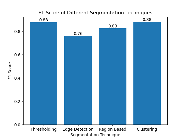
Although many recent approaches for image segmentation are emerging, traditional segmentation techniques such as thresholding, edge detection, region-based methods, and clustering can be very useful when applied to datasets such as the MIVIA HEp-2 image dataset.
Each method has its strength:
By evaluating these methods using F1 scores, we understand the trade-offs each of these models has. These methods may not be as sophisticated as what is developed in the newest models of deep learning, but they are still fast, interpretable, and serviceable in a broad range of applications.
Thanks for reading! I hope this exploration of traditional image segmentation techniques inspires your next project. Feel free to share your thoughts and experiences in the comments below!
以上が画像セグメンテーションをマスターする: デジタル時代でも伝統的な技術がどのように輝き続けるのかの詳細内容です。詳細については、PHP 中国語 Web サイトの他の関連記事を参照してください。


![[Web フロントエンド] Node.js クイック スタート](https://img.php.cn/upload/course/000/000/067/662b5d34ba7c0227.png)


