Large models can also be sliced, and Microsoft SliceGPT greatly increases the computational efficiency of LLAMA-2

Large-scale language models (LLM) usually have billions of parameters and are trained on trillions of tokens. However, such models are very expensive to train and deploy. In order to reduce computational requirements, various model compression techniques are often used.

These model compression techniques can generally be divided into four categories: distillation, tensor decomposition (including low-rank factorization), pruning and quantization. Pruning methods have been around for some time, but many require recovery fine-tuning (RFT) after pruning to maintain performance, making the entire process costly and difficult to scale.

Researchers at ETH Zurich and Microsoft have proposed a solution to this problem, called SliceGPT. The core idea of ​​this method is to reduce the embedding dimension of the network by deleting rows and columns in the weight matrix to maintain the performance of the model. The emergence of SliceGPT provides an effective solution to this problem.

The researchers noted that with SliceGPT, they were able to compress large models in a few hours using a single GPU, even without RFT, while remaining competitive in both generation and downstream tasks. force performance. Currently, the research has been accepted by ICLR 2024.

• ##Paper title: SLICEGPT: COMPRESS LARGE LANGUAGE MODELS BY DELETING ROWS AND COLUMNS
• Paper link: https://arxiv.org/pdf/2401.15024.pdf

The pruning method works by setting certain elements of the weight matrix in the LLM to zero and selectively updating surrounding elements to compensate. This results in a sparse pattern that skips some floating point operations in the forward pass of the neural network, thus improving computational efficiency.

The degree of sparsity and sparsity mode are factors that determine the relative improvement in computing speed. When the sparse mode is more reasonable, it will bring more computational advantages. Unlike other pruning methods, SliceGPT prunes by cutting off (cutting off!) entire rows or columns of the weight matrix. Before resection, the network undergoes a transformation that keeps the predictions unchanged but allows for slightly affected shearing processes.

The result is that the weight matrix is ​​reduced, signal transmission is weakened, and the dimension of the neural network is reduced.

Figure 1 below compares the SliceGPT method with existing sparsity methods.

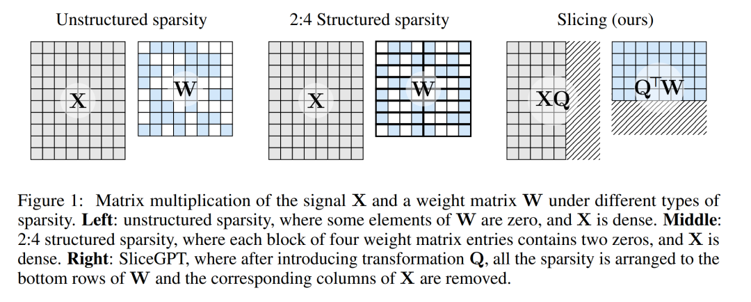
Through extensive experiments, the author found that SliceGPT can remove multiple pixels for LLAMA-2 70B, OPT 66B and Phi-2 models. up to 25% of the model parameters (including embeddings) while maintaining 99%, 99%, and 90% of the zero-shot task performance of the dense model, respectively.

The model processed by SliceGPT can run on fewer GPUs and faster without any additional code optimization: on a 24GB consumer GPU, the author will LLAMA-2 70B reduced the total inference computation to 64% of the dense model; on the 40GB A100 GPU, they reduced it to 66%.

In addition, they also proposed a new concept, computational invariance in Transformer networks, which makes SliceGPT possible.

SliceGPT in detail

The SliceGPT method relies on the computational invariance inherent in the Transformer architecture. This means that you can apply an orthogonal transformation to the output of one component and then undo it in the next component. The authors observed that RMSNorm operations performed between network blocks do not affect the transformation: these operations are commutative.

In the paper, the author first introduces how to achieve invariance in a Transformer network with RMSNorm connections, and then explains how to convert a network trained with LayerNorm connections to RMSNorm. Next, they introduce the method of using principal component analysis (PCA) to calculate the transformation of each layer, thereby projecting the signal between blocks onto its principal components. Finally, they show how removing minor principal components corresponds to cutting off rows or columns of the network.

Computational invariance of the Transformer network

Use Q to represent the orthogonal matrix:

• Note that multiplying a vector x by Q does not change the norm of the vector, since in this work the dimensions of Q always match the embedding dimensions of transformer D.

Assume that X_ℓ is the output of a block of transformer. After being processed by RMSNorm, it is input to the next block in the form of RMSNorm (X_ℓ). If you insert a linear layer with an orthogonal matrix Q before RMSNorm and Q^⊤ after RMSNorm, the network will remain unchanged because each row of the signal matrix is ​​multiplied by Q, normalized and multiplied by Q^ ⊤. Here we have:

Now, since each attention or FFN block in the network performs a linear operation on the input and output, we can The additional operations Q are absorbed into the linear layer of the module. Since the network contains residual connections, Q must also be applied to the outputs of all previous layers (up to the embedding) and all subsequent layers (up to the LM Head).

An invariant function refers to a function whose input transformation does not cause the output to change. In this article's example, any orthogonal transformation Q can be applied to the transformer's weights without changing the result, so the calculation can be performed in any transformation state. The authors call this computational invariance and define it in the following theorem.

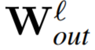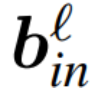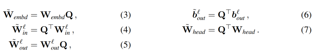
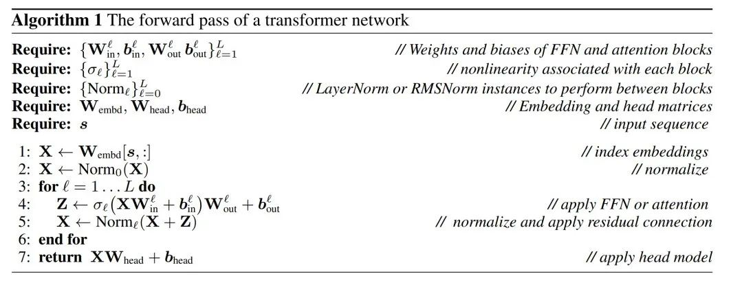
Theorem 1: Let and be the weight matrix of the linear layer of the ℓ linear layer of the transformer network connected by RMSNorm, , 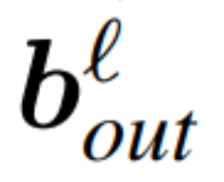is the corresponding offset (if any), W_embd and W_head are the embedding matrix and head matrix. Assume Q is an orthogonal matrix with dimension D, then the following network is equivalent to the original transformer network:

Copy input bias and head bias:

It can be proved by Algorithm 1 that the converted network calculates the same result as the original network.

##LayerNorm Transformer can be converted to RMSNorm

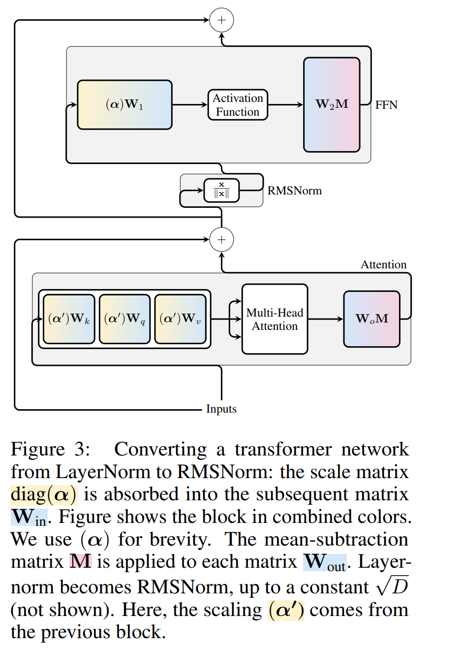
Transformer Computational invariance of networks only applies to RMSNorm connected networks. Before processing a network using LayerNorm, the authors first convert the network to RMSNorm by absorbing linear blocks of LayerNorm into adjacent blocks.

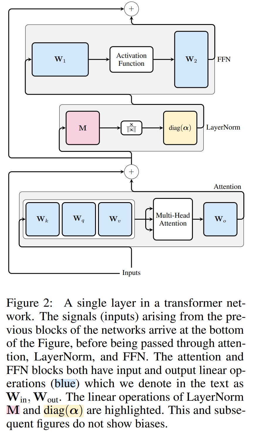
Figure 3 shows this transformation of the Transformer network (see Figure 2). In each block, the authors multiply the output matrix W_out with the mean subtraction matrix M, which takes into account the mean subtraction in subsequent LayerNorm. The input matrix W_in is premultiplied by the proportion of the previous LayerNorm block. The embedding matrix W_embd must undergo mean subtraction, and W_head must be rescaled according to the proportion of the last LayerNorm. This is a simple change in the order of operations and will not affect the network output.

Transformation of each block

Now that every LayerNorm in the transformer has been converted to RMSNorm, any Q can be selected to modify the model. The author's original plan was to collect signals from the model, use these signals to construct an orthogonal matrix, and then delete parts of the network. They quickly discovered that the signals from different blocks in the network were not aligned, so they needed to apply a different orthogonal matrix, or Q_ℓ, to each block.

If the orthogonal matrix used in each block is different, the model will not change, and the proof method is the same as Theorem 1, except for line 5 of Algorithm 1. Here you can see that the output of the residual connection and the block must have the same rotation. In order to solve this problem, the author modifies the residual connection by linearly transforming the residual .

Figure 4 shows how different rotations can be applied to different blocks by performing additional linear operations on the residual connections. Unlike modifications to the weight matrix, these additional operations cannot be precomputed and add a small (D × D) overhead to the model. Still, these operations are needed to cut away the model, and you can see that the overall speed does increase.

To calculate the matrix Q_ℓ, the author used PCA. They select a calibration dataset from the training set, run it through the model (after converting the LayerNorm operation to RMSNorm), and extract the orthogonal matrix for that layer. More precisely, if they use the output of the transformed network to calculate the orthogonal matrix for the next layer. More precisely, if is the output of the ℓ-th RMSNorm module for the i-th sequence in the calibration data set, calculate:

And set Q_ℓ as the eigenvector of C_ℓ, sorted in descending order of eigenvalues.

Excision

The goal of principal component analysis is usually to obtain the data matrix X and calculate Low-dimensional representation Z and approximate reconstruction :

##where Q is the feature vector of , D is a D × D small deletion matrix (containing D small columns of D × D homotopic matrices), used to delete some columns on the left side of the matrix. The reconstruction is L_2 optimal in the sense that QD is a linear map that minimizes .

When applying PCA to the inter-block signal matrix Operation. In the above operation, this matrix has been multiplied by Q. The author removed the row of W_in and the columns of W_out and W_embd. They also removed rows and columns of the matrix inserted into the residual connection (see Figure 4).

Experimental results

Generation task

The author conducted a performance evaluation on the OPT and LLAMA-2 model series of different sizes after being trimmed by SliceGPT and SparseGPT in the WikiText-2 data set. Table 1 shows the complexity retained after different levels of pruning of the model. Compared to the LLAMA-2 model, SliceGPT showed superior performance when applied to the OPT model, which is consistent with the author's speculation based on the analysis of the model spectrum.

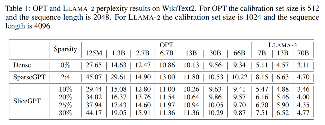
The performance of SliceGPT will improve as the model size increases. SparseGPT 2:4 mode performs worse than SliceGPT at 25% clipping for all LLAMA-2 series models. For OPT, it can be found that the sparsity of the model with 30% resection ratio is better than that of 2:4 in all models except the 2.7B model.

Zero-sample task

The author used five tasks: PIQA, WinoGrande, HellaSwag, ARC-e and ARCc to evaluate SliceGPT on zero-sample Performance on the task, they used LM Evaluation Harness as the default parameter in the evaluation.

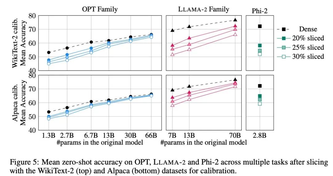
Figure 5 shows the average scores achieved by the tailored model on the above tasks. The upper row of the figure shows the average accuracy of SliceGPT in WikiText-2, and the lower row shows the average accuracy of SliceGPT in Alpaca. Similar conclusions can be observed from the results as in the generation task: the OPT model is more adaptable to compression than the LLAMA-2 model, and the larger the model, the less obvious the decrease in accuracy after pruning.

The author tested the effect of SliceGPT on a small model like Phi-2. The trimmed Phi-2 model performs comparably to the trimmed LLAMA-2 7B model. The largest OPT and LLAMA-2 models can be compressed efficiently, and SliceGPT only loses a few percentage points when removing 30% from the 66B OPT model.

The author also conducted recovery fine-tuning (RFT) experiments. A small number of RFTs were performed on the trimmed LLAMA-2 and Phi-2 models using LoRA.

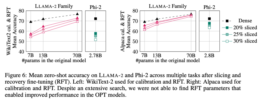
The experimental results are shown in Figure 6. It can be found that there are significant differences in the results of RFT between the WikiText-2 and Alpaca data sets, and the model shows better performance in the Alpaca data set. The authors believe that the reason for the difference is that the tasks in the Alpaca dataset are closer to the baseline tasks.

For the largest LLAMA-2 70B model, after pruning 30% and then performing RFT, the final average accuracy in the Alpaca data set was 74.3%, and the accuracy of the original dense model was 76.6%. The tailored model LLAMA-2 70B retains approximately 51.6B parameters and its throughput is significantly improved.

The author also found that Phi-2 was unable to recover the original accuracy from the pruned model in the WikiText-2 data set, but it could recover a few percentage points in the Alpaca data set. Accuracy. Phi-2, clipped by 25% and RFTed, has an average accuracy of 65.2% in the Alpaca dataset, and the accuracy of the original dense model is 72.2%. The trimmed model retains 2.2B parameters and retains 90.3% of the accuracy of the 2.8B model. This shows that even small language models can be pruned effectively.

Benchmark throughput

Different from traditional pruning methods, SliceGPT is in matrix (Structural) sparsity is introduced in: the entire column X is cut off, reducing the embedding dimension. This approach both enhances the computational complexity (number of floating point operations) of the SliceGPT compression model and improves data transfer efficiency.

On an 80GB H100 GPU, set the sequence length to 128 and batch-double the sequence length to find the maximum throughput until the GPU memory is exhausted or throughput drops. The authors compared the throughput of 25% and 50% pruned models to the original dense model on an 80GB H100 GPU. Models trimmed by 25% achieved up to 1.55x throughput improvement.

With 50% clipping, the largest model achieves substantial increases in throughput of 3.13x and 1.87x using a single GPU. This shows that when the number of GPUs is fixed, the throughput of the pruned model will reach 6.26 times and 3.75 times respectively of the original dense model.

After 50% pruning, although the complexity retained by SliceGPT in WikiText2 is worse than SparseGPT 2:4, the throughput far exceeds the SparseGPT method. For models sized 13B, throughput may also improve for smaller models on consumer GPUs with less memory.

Inference time

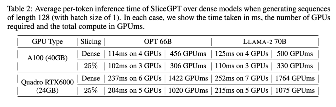
The author also studied the end-to-end model compression using SliceGPT terminal running time. Table 2 compares the time required to generate a single token for the OPT 66B and LLAMA-2 70B models on Quadro RTX6000 and A100 GPUs. It can be found that on the RTX6000 GPU, after trimming the model by 25%, the inference speed is increased by 16-17%; on the A100 GPU, the speed is increased by 11-13%. For LLAMA-2 70B, the amount of computation required using the RTX6000 GPU is reduced by 64% compared to the original dense model. The author attributes this improvement to SliceGPT's replacement of the original weight matrix with a smaller weight matrix and the use of dense kernels, which cannot be achieved by other pruning schemes.

The authors stated that at the time of writing, their baseline SparseGPT 2:4 was unable to achieve end-to-end performance improvements. Instead, they compared SliceGPT to SparseGPT 2:4 by comparing the relative time of each operation in the transformer layer. They found that for large models, SliceGPT (25%) was competitive with SparseGPT (2:4) in terms of speed improvement and perplexity.

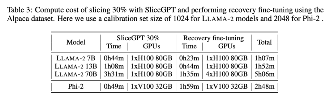
Computational cost

##All LLAMA-2, OPT and Phi-2 models Slicing can take 1 to 3 hours on a single GPU. As shown in Table 3, with recovery fine-tuning, all LMs can be compressed within 1 to 5 hours.

For more information, please refer to the original paper.

The above is the detailed content of Large models can also be sliced, and Microsoft SliceGPT greatly increases the computational efficiency of LLAMA-2. For more information, please follow other related articles on the PHP Chinese website!