

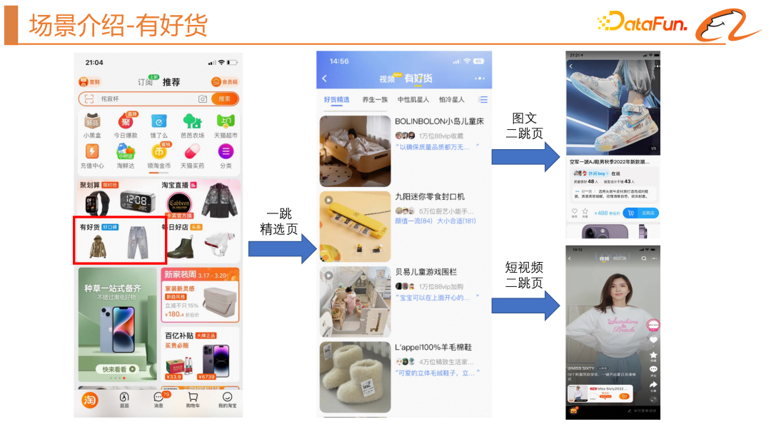
##First of all Let’s introduce the scenario involved in this article - the “good goods are available” scenario. Its location is in the four-square grid on Taobao's homepage, which is divided into a one-hop selection page and a two-hop acceptance page. There are two main forms of acceptance pages, one is the image and text acceptance page, and the other is the short video acceptance page. The goal of this scenario is mainly to provide users with satisfactory goods and drive the growth of GMV, thereby further leveraging the supply of experts.
Next comes the focus of this article, popularity bias. What is popularity bias? Why does popularity bias occur?
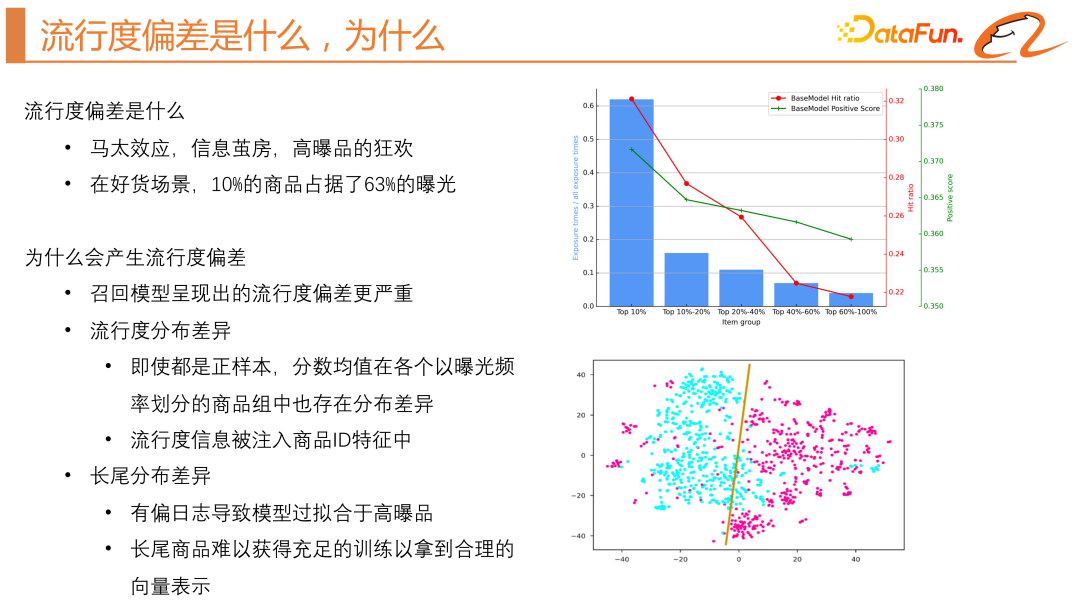
Popularity bias has many aliases, such asMatthew effect, information cocoon room,Intuitively speaking, it is a carnival of high-explosive products. The more popular the product, the easier it is to be exposed. This will result in high-quality long-tail products or new products created by experts not having a chance to be exposed. There are two main harms. The first point is the lack of user personalization. The second point is that the new products created by the experts do not receive enough exposure, which reduces the sense of participation of the experts. Therefore, we hope to alleviate the popularity bias.
As can be seen from the blue histogram on the right side of the above figure, the top 10% exposed products accounted for 63% of the exposure on a certain day, which proves that in The Matthew effect is very serious when there are good goods.
Next, let’s attribute why popularity bias occurs. . First, we need to clarify why we do the work of mitigating popularity bias in recall truncation. The ranking model fits the CTR of the product, and its training samples include positive samples and negative samples. Products with higher CTR are more likely to gain exposure. But in the recall stage, we usually use the twin-tower model. Its negative samples are usually generated in two ways. The first is global random negative sampling, and the second is intra-batch negative sampling. Intra-batch negative sampling is the same A batch takes other exposure logs of positive samples as negative samples, so it can alleviate the Matthew effect to a certain extent. However, through experiments, we found that the actual online efficiency effect of global negative sampling will be better. However, global random negative sampling in recommender systems may lead to popularity bias because it only provides positive feedback to the model. This bias may be attributed to popularity distribution differences and prior knowledge interference, i.e., users tend to click on more popular items. Therefore, the model may preferentially recommend popular items regardless of their relevance.
We also analyzed the differences in popularity distribution, as shown in the green line on the right side of the figure above, by grouping the products according to exposure frequency and Calculating the average score of positive samples for each group, it was found that even if all samples are positive samples, the average score decreases with the frequency of exposure. There are differences in popularity distribution and long-tail distribution when training recommendation system models. The model will tend to inject popularity information into the ID features of items, resulting in differences in popularity distribution. The number of training times obtained by high-explosive products is much larger than that of long-tail products, making the model overfitting for high-explosive products, and it is difficult for long-tail products to obtain sufficient training and reasonable vector representation. As shown in the TSN chart on the right side of the figure above, the blue dots represent the product vectors of high-exposure products, while the red dots represent the product vectors of long-tail products, showing a significant difference in distribution. And as shown in the red line on the right side of the figure above, the hit ratio will also decrease as the number of exposures decreases. Therefore, we attribute the popularity bias to the difference in popularity distribution and the difference in long-tail distribution.
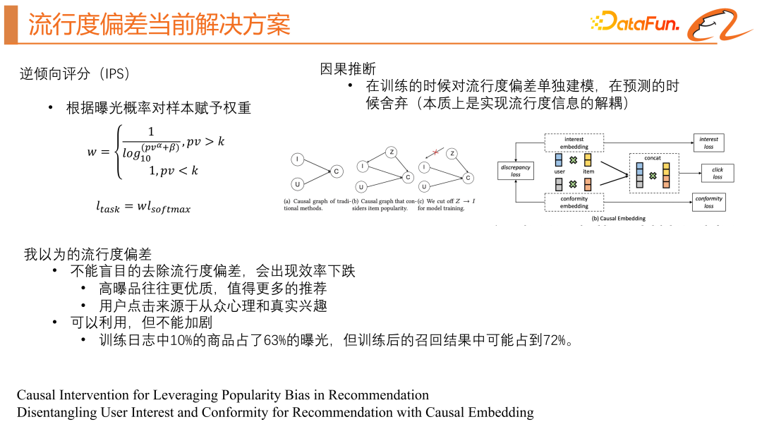
Current industry solutionsThere are two main types, namely inverse propensity score (IPS) and causal inference.
Generally speaking, it is to lower the weight of high-exposure probability products in the main task loss function to Avoid paying too much attention to products with high exposure probability, so that you can pay more equal attention to the entire positive sample distribution. However, this method requires predicting the exposure probability in advance, which is unstable and prone to failure or large fluctuations.
We need to construct a causal diagram, where i represents product characteristics and u represents users Features, c represents the click probability. This picture shows that user features and product features are input into the model to predict the click rate. If we also take the popularity bias into this model, represented by z, it will not only affect the click-through rate, but also affect the feature representation of the product i. The method of causal inference is to try to block the impact of z on i.
The simpler method is to use some statistical characteristics of the product to obtain a separate bias tower. At this time, the model will output two points, one is the true click-through rate , and the other is the popularity score of the product. When making online predictions, the popularity score of the product will be removed to achieve decoupling of the popularity deviation.
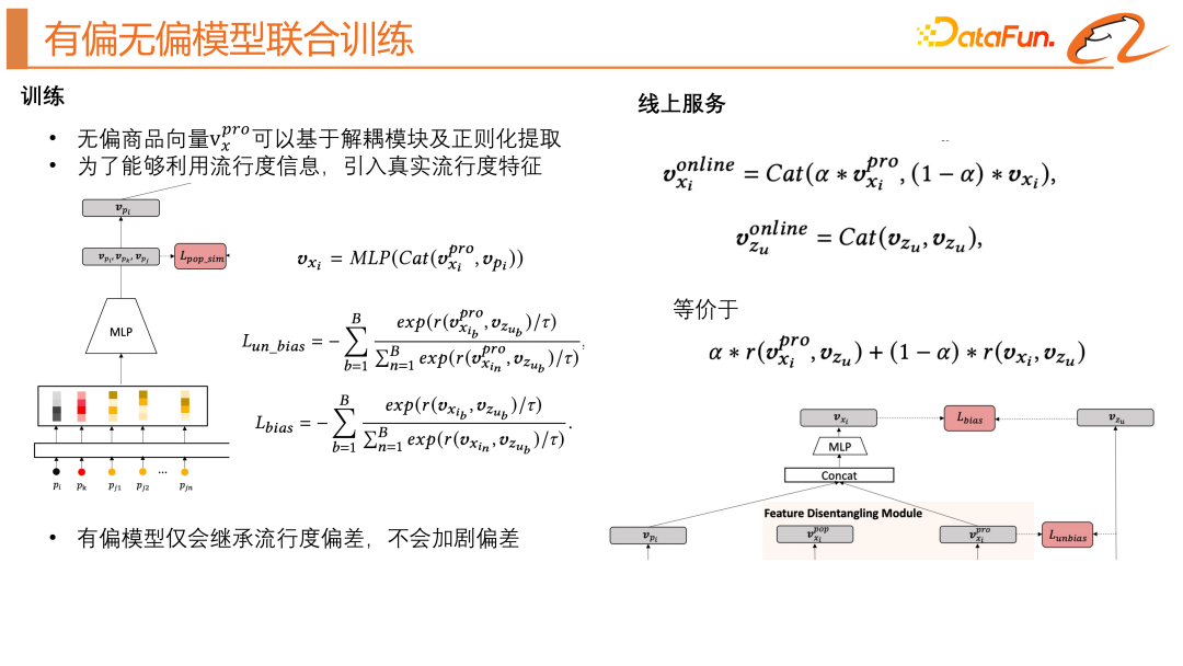
#The second method is to attribute user clicks into two categories, one is herd interest and the other is real interest, and build joint training of samples respectively. It is equivalent to obtaining two models, one model to obtain the user's herd interest score, and one model to obtain the user's true interest score. There are actually problems with causal inference. It solves the difference in popularity distribution, but it cannot solve the problem of lack of training data for long-tail products. Current solutions tend to remove popularity bias, but this may not always be beneficial for recommender systems that need the "Matthew Effect" to survive. Therefore, we recommend not to completely remove the popularity bias in the recommendation system, because popular items are usually of higher quality, and users also have both a herd mentality and a real interest. Completely removing the popularity bias will affect the satisfaction of users' herd interests. Popularity bias should be utilized rationally and not exacerbated.
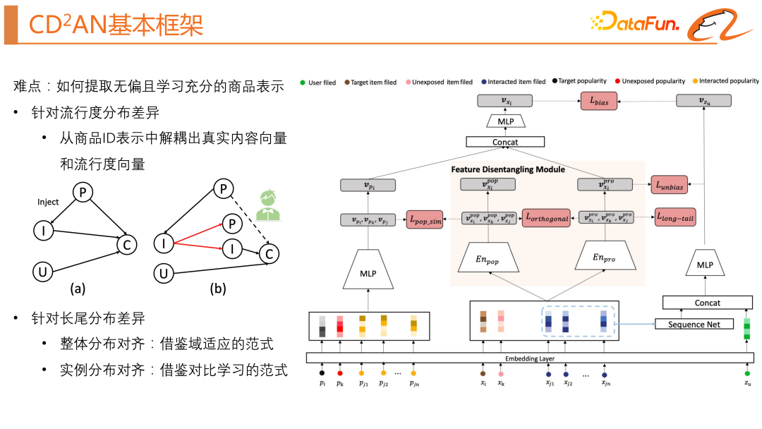
## The work we are exploring this time is how to reasonably use the popularity bias. To use the popularity bias reasonably, we need to solve a difficulty: "How to extract an unbiased and fully learned product representation?" In view of the difference in popularity distribution, we need to Decouple the real content vector and popularity vector from the product ID. To address long-tail distribution differences, we draw on the paradigm of domain adaptation to align the overall distribution, and draw on the paradigm of contrastive learning to align the instance distributions.
Let’s first introduce the basic structure of the base model. The base model is actually a classic two-tower model. Next, we will introduce in detail how we solve the two problems mentioned earlier (popularity distribution difference and long-tail distribution difference).
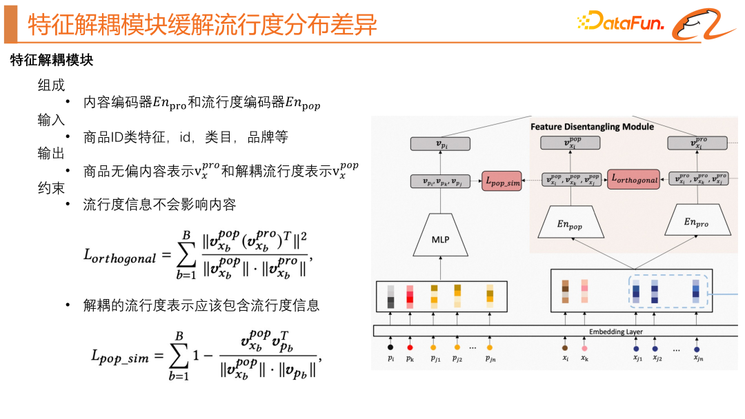
The feature decoupling module is a solution proposed in this article to solve the problem of popularity bias in recommendation systems. This module reduces the impact of popularity on item vector representation by separating popularity information from attribute information in item vector representation. Specifically, this module includes a popularity encoder and an attribute encoder, and learns the attribute and popularity vector representation of each item through a combination of multi-layer perceptrons. The input of this module is the attribute characteristics of the item, such as item ID, item category, brand, etc., as shown in the right part of the model structure above. There will be two constraints here, including orthogonal regularization and popularity similarity regularization, aiming to separate the popularity information from the item attribute information. Among them, through popularity similarity regularization, the module is encouraged to align the popularity information embedded in item attributes with the real popularity information, while through orthogonal regularization, the module is encouraged to retain different information in the encoding, thereby achieving separated popularity. degree information and item attribute information.
We also need a module to learn the true popularity, as shown in the left part of the model structure above. Its input is mainly the statistical characteristics of the product. Then go through an MLP to get the true popularity representation.
##Next, we want to solve the problem of long-tail distribution differences.
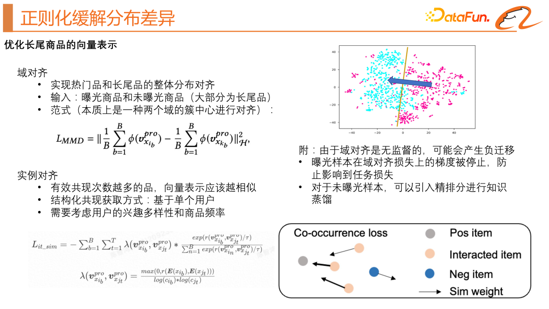
We draw on the idea of transfer learning to achieve distribution alignment of popular products and long-tail products. In the original two-tower model, we introduced an unexposed product and used the MMD loss function (as shown in the upper left of the figure above). This loss function hopes that the cluster centers of the popular product domain and the long-tail product domain are as close as possible, as shown above As shown in the schematic diagram on the upper right side of the figure. Since this kind of domain alignment is unsupervised and may produce negative transfer, we have made the following optimizations: the gradient of the exposed samples on the domain alignment loss is stopped to prevent it from affecting the task loss; for unexposed samples, fine ranking is introduced. Knowledge distillation.We also draw on the idea of instance alignment, hoping to learn better product vector representations. The main idea is that the more effective co-occurrences of products, the more similar the vector representations will be. The difficulty here is how to construct the pair. Such a pair naturally exists in the product sequence where the user has past behavior. Taking a user as an example, a sample contains a user's behavior sequence and target products. Then the target product and each product in the user's behavior sequence can form a co-occurring pair. On the basis of the classic contrastive learning loss function, we also consider the user's interest diversity and product frequency. The specific loss function formula can be seen in the lower left part of the above figure.
We can look at an intuitive diagram, as shown in the lower right of the above figure. The gray points are the target products, the orange points are the user's behavior sequence, and the blue points are the negative values obtained by our random negative sampling. sample. We hope to learn from the contrastive learning method to constrain each product in the user behavior sequence to be close to the target product.3. Biased and unbiased joint training
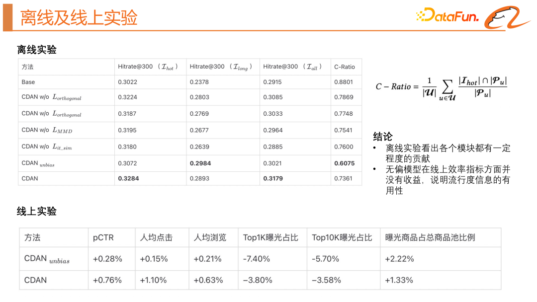
##The above picture shows the offline and online effects of this model. In offline experiments, we introduced the C-Ratio indicator to measure how many items in the recall results are highly exposed items. Through offline experiments, we can see that each module contributes to a certain extent. The unbiased model has no gain in online efficiency indicators, indicating that popularity information is useful, and we still need to use a biased model to utilize popularity information.

Finally, we made a visual display of the model results. We found that the new model structure can indeed align the distribution of high-explosive products and long-tail products. The decoupled popularity representation vector and the unbiased content representation of the product have almost no intersection, and products of the same purpose can have closer relationships. By adjusting α, the model can directionally fit the user's herd interests and real interests.
The title of the paper shared today is "Co-training Disentangled Domain Adaptation Network for Leveraging Popularity Bias in Recommenders".
A1: Generated offline. For one sample, we can get the target positive sample and the corresponding category, and then randomly sample several and target positive samples offline. Products of the same category are attached to the training samples.
#A3: Use the fine ranking model to score the sample offline and use it as a feature. The performance is not bad.
#A4: No, there is a high probability that this is still a high-explosive product. We are using the results of random sampling under the same global category.
The above is the detailed content of The Secret of Accurate Recommendation: Detailed Explanation of Alibaba's Decoupled Domain Adaptation Unbiased Recall Model. For more information, please follow other related articles on the PHP Chinese website!


