


Usually, it is very common to have outliers in the data distribution we process, and many algorithms can handle outliers, and EllipticalEnvelope is built directly into Sklearn An example of. The advantage of this algorithm is that it performs very well in detecting outliers in normally distributed (Gaussian) features:
import numpy as np
from sklearn.covariance import EllipticEnvelope

# 创建一个样本正态分布
X = np.random.normal(loc=5, scale=2, size=50).reshape(-1, 1)

# 拟合估计量
ee = EllipticEnvelope(random_state=0)
_ = ee.fit(X)

# 测试
test = np.array([6, 8, 20, 4, 5, 6, 10, 13]).reshape(-1, 1)

# Predict返回1作为内嵌值,返回-1作为异常值
>>> ee.predict(test)

array([ 1,  1, -1,  1,  1,  1, -1, -1])
To verify the evaluation results, we generated a mean with a mean of 5 and a standard deviation of 2 normal distribution. After training is complete, pass some random numbers to its prediction method. This method returns -1 to indicate outliers in the test, i.e. 20, 10, 13.
When we do data mining and feature engineering, selecting the features that are most helpful for prediction is a necessary step to prevent overfitting and reduce model complexity. One of the most robust algorithms provided by Sklearn is Recursive Feature Elimination (RFE). It automatically finds the most important features by using cross-validation and discards the rest.
One advantage of this evaluator is that it is a wrapper - it can be used for any Sklearn algorithm that returns feature importance or coefficient scores. Here is an example on a synthetic dataset:
from sklearn.datasets import make_regression
from sklearn.feature_selection import RFECV
from sklearn.linear_model import Ridge

# 构建一个合成数据集
X, y = make_regression(n_samples=10000, n_features=15, n_informative=10)

# 初始化和拟合选择器
rfecv = RFECV(estimator=Ridge(), cv=5)
_ = rfecv.fit(X, y)

# 转换特性阵列
>>> rfecv.transform(X).shape
(10000, 10)
The dataset has 15 features, 10 of which are informative and the rest are redundant. We fit 5-fold RFECV with ridge regression as the estimator. After training, transformation methods can be used to discard redundant features. Finally, call .shape to see that the evaluator has removed all 5 redundant features.
We all know that although random forests are very powerful, the risk of overfitting is very high. Therefore, Sklearn provides an alternative to RF called ExtraTrees (classifiers and regressors).
"Extra" This word does not refer to more trees, but refers to more randomness. This algorithm uses another tree similar to a decision tree. The only difference is that instead of calculating segmentation thresholds when building each tree, these thresholds are randomly drawn for each feature and the best threshold is selected as the segmentation rule. This allows for reduced variance at the cost of a slightly increased bias:
from sklearn.ensemble import ExtraTreesRegressor, RandomForestRegressor
from sklearn.model_selection import cross_val_score
from sklearn.tree import DecisionTreeRegressor

X, y = make_regression(n_samples=10000, n_features=20)

# 决策树
clf = DecisionTreeRegressor(max_depth=None, min_samples_split=2, random_state=0)
scores = cross_val_score(clf, X, y, cv=5)
>>> scores.mean()
0.6376080094392635

# 随机森林
clf = RandomForestRegressor(
    n_estimators=10, max_depth=None, min_samples_split=2, random_state=0
)
scores = cross_val_score(clf, X, y, cv=5)
>>> scores.mean()
0.8446103607404536

# ExtraTrees
clf = ExtraTreesRegressor(
    n_estimators=10, max_depth=None, min_samples_split=2, random_state=0
)
scores = cross_val_score(clf, X, y, cv=5)
>>> scores.mean()
0.8737373931608834As the results show, ExtraTreesRegressor outperforms Random Forest on synthetic datasets.
If you are looking for a more robust and advanced imputation technology than SimpleImputer, Sklearn Once again your support is provided. The impute sub-package includes two model-based impute algorithms KNNImputer and IterativeImputer.
As the name suggests, KNNImputer uses the k-Nearest-Neighbors algorithm to find the best replacement for missing values:
from sklearn.impute import KNNImputer
# 代码取自Sklearn用户指南
X = [[1, 2, np.nan],
     [3, 4, 3],
     [np.nan, 6, 5],
     [8, 8, 7]]
imputer = KNNImputer(n_neighbors=2)
imputer.fit_transform(X)Output:
array([[1. , 2. , 4. ],
[3. , 4. , 3. ],
[5.5, 6. , 5. ],
[ 8. , 8. , 7. ]])
Another more robust algorithm is IterativeImputer. It finds missing values by modeling the missing values of each feature as a function of other features. This process is completed in a step-by-step cycle. At each step, one feature with missing values is selected as the target (y) and the rest as the feature array (X). Then, use the regression function to predict missing values in y, and continue this process for each feature up to max_iter times (a parameter of IterativeImputer).
Therefore, multiple predictions are generated for a missing value. The benefit of this approach is to treat each missing value as a random variable and combine it with the inherent uncertainty
from sklearn.experimental import enable_iterative_imputer
from sklearn.impute import IterativeImputer
from sklearn.linear_model import BayesianRidge
imp_mean = IterativeImputer(estimator=BayesianRidge())
imp_mean.fit([[7, 2, 3],
              [4, np.nan, 6],
              [10, 5, 9]])

X = [[np.nan, 2, 3],
     [4, np.nan, 6],
     [10, np.nan, 9]]
imp_mean.transform(X)Output:
array([[ 6.95847623, 2. , , 3. ],
[ 4. , , 2.6000004, 6. ],
[10. , 4.99999933 , 9. ]])
The results show that using IterativeImputer The missing value filling algorithm’s BayesianRidge and ExtraTree algorithm performance effects are even better.
Although it is very common for outliers to exist in data distributions under normal circumstances, the presence of outliers can seriously undermine the predictions of any model. Many outlier detection algorithms discard outliers and mark them as missing. While this aids model learning, it completely removes the impact of outliers on the distribution.
另一种算法是 HuberRegressor 回归算法。它不是完全去除它们,而是在拟合数据期间给予异常值更小的权重。它有超参数 epsilon 来控制样本的数量,这些样本应该被归类为异常值。参数越小,对异常值的鲁棒性越强。它的API与任何其他线性回归函数相同。下面,你可以看到它与贝叶斯岭回归器在一个有大量异常值的数据集上的比较:
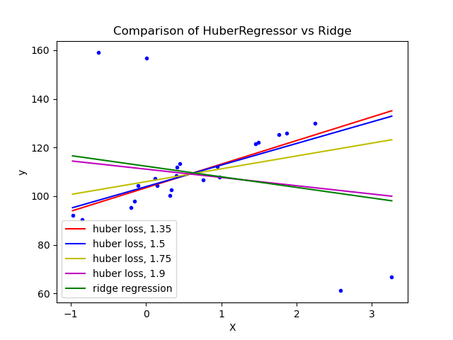
可以看到,设置参数 epsilon 为 1.35 1.5, 1.75 的 huberregressionor 算法设法捕获不受异常值影响的最佳拟合线。
Sklearn 中可以使用 plot_tree 函数绘制单个决策树的结构。这个特性可能对刚开始学习基于树的模型和集成模型的初学者很方便,通过该方法,对决策树的决策过程可视化,对其决策过程和原理更加一目了然。
from sklearn.datasets import load_iris
from sklearn.tree import DecisionTreeClassifier, plot_tree

iris = load_iris()
X, y = iris.data, iris.target
clf = DecisionTreeClassifier()
clf = clf.fit(X, y)

plt.figure(figsize=(15, 10), dpi=200)
plot_tree(clf, feature_names=iris.feature_names,
               class_names=iris.target_names);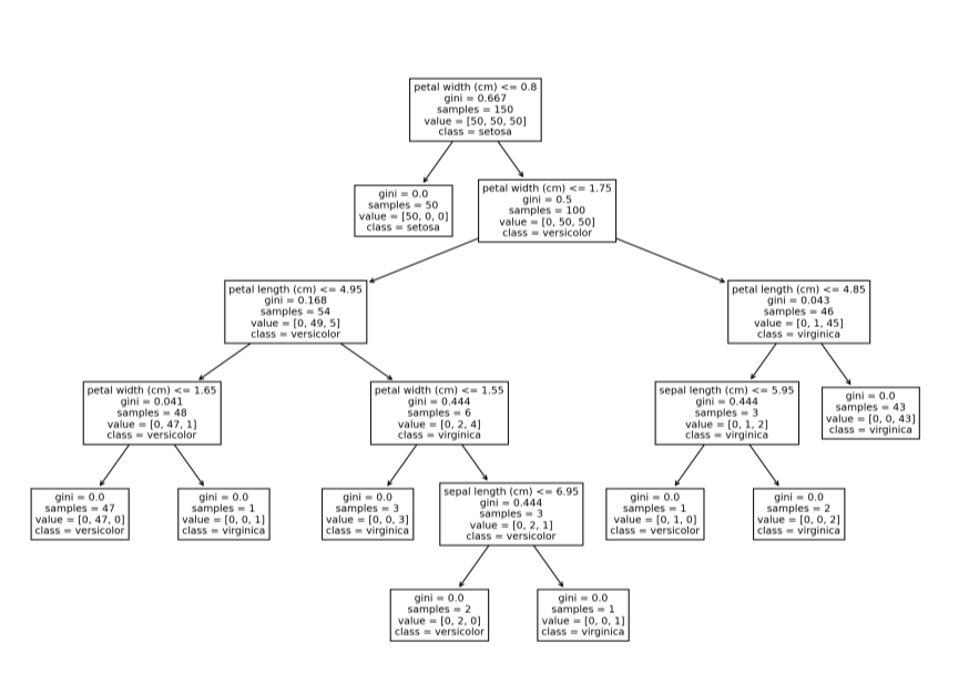
还有其他绘制树的方法,比如 Graphviz。
尽管感知机是一个奇特的名字,但它是一个简单的线性二进制分类器。算法的定义特征是适合大规模学习,默认为:
它不需要学习速率。
不要实现正则化。
它只在分类错误的情况下更新模型。
它等价于 SGDClassifier,loss='perceptron', eta0=1, learning_rate="constant", penalty=None ,但略快:
from sklearn.datasets import make_classification
from sklearn.linear_model import Perceptron
# 创建一个更大的数据集
X, y = make_classification(n_samples=100000, n_features=20, n_classes=2)
# Init/Fit/Score
clf = Perceptron()
_ = clf.fit(X, y)
clf.score(X, y)
输出:
0.91928
Sklearn 中另一个基于模型的特征选择模型是 SelectFromModel。它不像RFECV那样健壮,但由于它具有较低的计算成本,可以作为大规模数据集的一个很好的选择。它也是一个包装器模型,适用于任何具有 .feature_importance_ 或 .coef_ 属性的模型:
from sklearn.feature_selection import SelectFromModel

# 创建一个包含40个无信息特征的数据集
X, y = make_regression(n_samples=int(1e4), n_features=50, n_informative=10)

# 初始化选择器并转换特性数组
selector = SelectFromModel(estimator=ExtraTreesRegressor()).fit(X, y)

selector.transform(X).shape
输出:
(10000, 8)
如结果所示,算法成功地删除了所有40个冗余特征。
总所周知,混淆矩阵是用于评估分类问题的常用方法。大多数我们通常使用的指标,如精度、召回率、F1、ROC AUC等等,都源于它。Sklearn中可以计算和绘制一个默认的混淆矩阵:
from sklearn.metrics import plot_confusion_matrix
from sklearn.model_selection import train_test_split

# 创建一个二元分类问题
X, y = make_classification(n_samples=200, n_features=5, n_classes=2)
X_train, X_test, y_train, y_test = train_test_split(
    X, y, test_size=0.5, random_state=1121218
)

clf = ExtraTreeClassifier().fit(X_train, y_train)
fig, ax = plt.subplots(figsize=(5, 4), dpi=100)
plot_confusion_matrix(clf, X_test, y_test, ax=ax);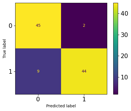
老实说,我不喜欢默认的混淆矩阵。它的格式是固定的—行是true labels,列是predictions label。第一行和第一列是负类,第二行和第二列是正类。有些人可能更喜欢不同格式的矩阵,可能是转置或翻转的。
例如,我喜欢将正类作为第一行和第一列。这有助于我更好地隔离 4 矩阵项 -- TP, FP, TN, FN。幸运的是,你可以用另一个函数 ConfusionMatrixDisplay 绘制自定义矩阵:
from sklearn.metrics import ConfusionMatrixDisplay, confusion_matrix

clf = ExtraTreeClassifier().fit(X_train, y_train)
y_preds = clf.predict(X_test)

fig, ax = plt.subplots(figsize=(5, 4), dpi=100)
cm = confusion_matrix(y_test, y_preds)
cmp = ConfusionMatrixDisplay(cm,
      display_labels=["Positive", "Negative"])
cmp.plot(ax=ax);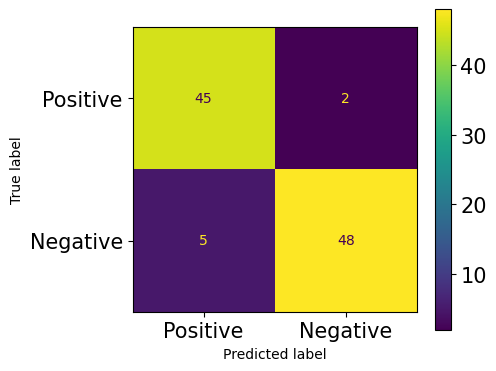
在传递给 ConfusionMatrixDisplay 之前,可以把 混淆矩阵cm 放在任何格式中。
一般情况下,如果有可用于其他类型分布的替代方案,则将目标(y)转换为正态分布是没有意义的。
例如,Sklearn 为目标变量提供了3种广义线性模型,分别是泊松、Tweedie或Gamma分布 ,而不是所期望的正态分布,poissonregressionor, TweedieRegressor 和 GammaRegressor 可以生成具有各自分布的目标的稳健结果。
除此之外,他们的api与任何其他Sklearn模型一样。可以将它们的概率密度函数绘制在同一坐标系上,以确定目标的分布是否与这三个分布相匹配。
例如,要查看目标是否遵循泊松分布,可以使用 Seaborn 的 kdeploy 绘制它的 PDF,并在相同的轴上使用 np.random_poisson 从 Numpy 中采样,绘制完美的泊松分布。
通常来说,基于树形模型和集合模型生成的结果更加稳健,同时在检测异常点方面也被证实是有效的。Sklearn 中的 IsolationForest 使用一个极端随机树 (tree.ExtraTreeRegressor) 来检测异常值。每个样本被分裂到树的不同分支上,每个分支根据选定的单一特征,在该特征的最大和最小值之间随机选择一个分裂值。
这种随机分区会在每棵树的根节点和终止节点之间产生明显更短的路径。
因此,当随机树组成的森林为特定样本共同产生更短的路径长度时,它们极有可能是异常——Sklearn用户指南。
from sklearn.ensemble import IsolationForest
X = np.array([-1.1, 0.3, 0.5, 100]).reshape(-1, 1)
clf = IsolationForest(random_state=0).fit(X)
clf.predict([[0.1], [0], [90]])
输出:
array([ 1, 1, -1])
许多线性模型需要在数值特征上进行一些转换才能使其服从正态分布。StandardScaler 和 MinMaxScaler 在大多数发行版中都比较适用。然而,当数据存在高偏度时,分布的核心指标,如平均值、中位数、最小值和最大值,就会受到影响。因此,简单的标准化和标准化对倾斜分布不起作用。
相反,Sklearn 实现中提供了一个名为 PowerTransformer的方法,它使用对数变换将任何倾斜的特征尽可能地转化为正态分布。考虑 Diamonds 数据集中的两个特征:
import seaborn as sns

diamonds = sns.load_dataset("diamonds")
diamonds[["price", "carat"]].hist(figsize=(10, 5));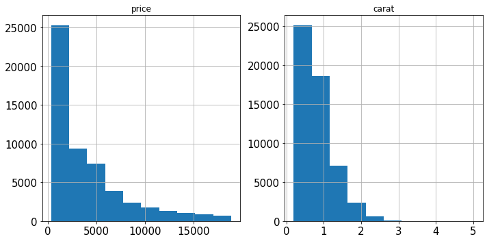
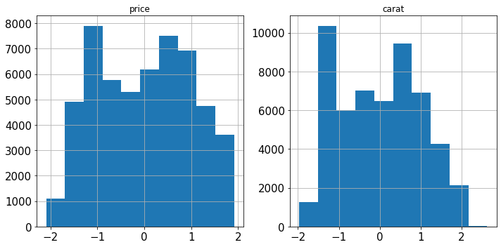
两者都严重倾斜。我们用对数变换 PowerTransformer来解决这个问题:
from sklearn.preprocessing import PowerTransformer

pt = PowerTransformer()
diamonds.loc[:, ["price", "carat"]] = pt.fit_transform(diamonds[["price", "carat"]])

diamonds[["price", "carat"]].hist(figsize=(10, 5));
Sklearn 中的另一个数字转换器是 RobustScaler,我们可以从它的名称猜出它的用途——可以以一种健壮到异常值的方式转换特性。如果一个特征中存在异常值,就很难使其服从正态分布,因为它们会严重扭曲均值和标准差。
与使用均值/标准不同,RobustScaler 使用中值和IQR(四分位数范围)来衡量数据,因为这两个指标都不会因为异常值而有偏差。
在 Sklearn 中,有一个用 make_pipeline 函数创建 Pipeline 实例的简写。该函数不需要为Pipeline中的每一步命名,而是只接受变形器和估计器并执行它的工作,从而不需要使代码那么长:
from sklearn.impute import SimpleImputer
from sklearn.pipeline import make_pipeline
from sklearn.preprocessing import StandardScaler

pipeline = make_pipeline(SimpleImputer(), StandardScaler(), ExtraTreesRegressor())
pipeline
Pipeline(steps=[('simpleimputer',
                  SimpleImputer()),
                ('standardscaler',
                  StandardScaler()),
                ('extratreesregressor',
ExtraTreesRegressor())])对于更复杂的场景,使用 ColumnTransformer,这有相同的问题——每个预处理步骤都应该命名,这会使代码变得冗长且不可读。Sklearn提供了与 make_pipeline 类似的函数:
import seaborn as sns
from sklearn.compose import make_column_transformer
from sklearn.preprocessing import OneHotEncoder

# 负载钻石数据集
diamonds = sns.load_dataset("diamonds")
X, y = diamonds.drop("price", axis=1), diamonds.price.values.reshape(-1, 1)

# 拆分数字和类别标签
num_cols = X.select_dtypes(include=np.number).columns
cat_cols = X.select_dtypes(exclude=np.number).columns

make_column_transformer((StandardScaler(), num_cols),
(OneHotEncoder(), cat_cols))ColumnTransformer(
transformers=[('standardscaler',
StandardScaler(),
Index(['carat', 'depth',
'table', 'x', 'y', 'z'],
dtype='object')),
('onehotencoder',
OneHotEncoder(),
Index(['cut', 'color',
'clarity'],
dtype='object'))]
)如上所示,使用 make_column_transformer 要短得多,并且它自己负责命名每个转换器步骤。
上文中,我们使用 select_dtypes 函数和 pandas DataFrames 的 columns 属性来拆分数值列和分类列。虽然这当然有效,但使用 Sklearn 有一个更灵活、更优雅的解决方案。
make_column_selector 函数创建一个可以直接传递到 ColumnTransformer 实例中的列选择器。它的工作原理与 select_dtypes 类似,甚至更好。它有 dtype_include 和 dtype_exclude 参数,可以根据数据类型选择列。如果需要自定义列筛选器,可以将正则表达式传递给 pattern,同时将其他参数设置为 None。下面是它的工作原理:
from sklearn.compose import make_column_selector

make_column_transformer(
    (StandardScaler(), make_column_selector(dtype_include=np.number)),
    (OneHotEncoder(), make_column_selector(dtype_exclude=np.number)),
)只是传递一个实例 make_column_selector 与由你设置相关参数,而不是传递一个列名称列表!
在我们刚学习机器学习时,常见的一个错误是使用 LabelEncoder 来编码有序的分类特征。注意到,LabelEncoder 一次只允许转换一个列,而不是像 OneHotEncoder 那样同时转换。你可能会认为 Sklearn 犯了一个错误!
实际上,LabelEncoder 应该只用于按照 LabelEncoder 文档中指定的方式对响应变量(y)进行编码。要编码特征数组(X),应该使用 OrdinalEncoder,它将有序分类列转换为具有(0, n_categories - 1) 类的特性。它在一行代码中跨所有指定列执行此操作,使得在管道中包含它成为可能。
from sklearn.preprocessing import OrdinalEncoder

oe = OrdinalEncoder()
X = [
    ["class_1", "rank_1"],
    ["class_1", "rank_3"],
    ["class_3", "rank_3"],
    ["class_2", "rank_2"],
]
oe.fit_transform(X)输出:
array([[0., 0.],
[0., 2.],
[2., 2.],
[1., 1.]])
Sklearn 内置了 50 多个指标,它们的文本名称可以在 Sklearn.metrics.scores.keys 中看到。在单个项目中,如果单独使用它们,则可能需要使用多个指标并导入它们。
从 sklearn.metrics 中导入大量指标可能会污染你的名称空间,使其变得不必要的长。一种解决方案是可以使用 metrics.get_scorer 函数使用其文本名称访问任何度量,而不需要导入它:
from sklearn.metrics import get_scorer

>>> get_scorer("neg_mean_squared_error")
make_scorer(mean_squared_error,
            greater_is_better=False)

>>> get_scorer("recall_macro")
make_scorer(recall_score,
            pos_label=None,
            average=macro)

>>> get_scorer("neg_log_loss")
make_scorer(log_loss,
            greater_is_better=False,
needs_proba=True)在 sklearn 的 0.24 版本中,引入了两个实验性超参数优化器:HalvingGridSearchCV 和 HalvingRandomSearchCV 类。
与它们详尽的同类 GridSearch 和 RandomizedSearch 不同,新类使用了一种称为连续减半的技术。 不是在所有数据上训练所有候选集,而是只将数据的一个子集提供给参数。通过对更小的数据子集进行训练,筛选出表现最差的候选人。每次迭代后,训练样本增加一定的因子,而可能的候选个数减少尽可能多的因子,从而获得更快的评估时间。
快多少呢?在我做过的实验中,HalvingGridSearch 比普通 GridSearch 快11倍,HalvingRandomSearch 甚至比 HalvingGridSearch 快10倍。
Sklearn在 sklearn.utils 中有一整套实用程序和辅助功能。Sklearn本身使用这个模块中的函数来构建我们使用的所有变形器transformers和估计器transformers。
这里有许多有用的方法,如 class_weight.compute_class_weight、estimator_html_repr、shuffle、check_X_y等。你可以在自己的工作流程中使用它们,使你的代码更像 Sklearn,或者在创建适合 Sklearn API 的自定义转换器和评估器时,它们可能会派上用场。
The above is the detailed content of What are the super practical hidden functions in Python Sklearn?. For more information, please follow other related articles on the PHP Chinese website!


![[Web front-end] Node.js quick start](https://img.php.cn/upload/course/000/000/067/662b5d34ba7c0227.png)


