


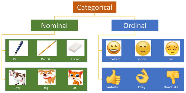
Categorical features refer to characteristics with values that fall within a finite set of categories, such as occupation and blood type.. Its original input is usually in the form of a string. Most algorithm models do not accept the input of numerical features. Numerical categorical features will be treated as numerical features, causing errors in the trained model.
Label Encoding uses a dictionary to associate each category label with an increasing integer, that is, generating a file named class Index into the instance array of _.
The LabelEncoder in Scikit-learn is used to encode categorical feature values, that is, to encode discontinuous values or text. It includes the following common methods:
fit(y): fit can be regarded as an empty dictionary, and y can be regarded as a word that is inserted into the dictionary.
fit_transform(y): It is equivalent to performing fit first and then transforming, that is, stuffing y into the dictionary and then transforming to get the index value.
inverse_transform(y): Obtain the original data based on the index value y.
transform(y): Transform y into an index value.
from sklearn.preprocessing import LabelEncoder le = LabelEncoder() city_list = ["paris", "paris", "tokyo", "amsterdam"] le.fit(city_list) print(le.classes_) # 输出为:['amsterdam' 'paris' 'tokyo'] city_list_le = le.transform(city_list) # 进行Encode print(city_list_le) # 输出为:[1 1 2 0] city_list_new = le.inverse_transform(city_list_le) # 进行decode print(city_list_new) # 输出为:['paris' 'paris' 'tokyo' 'amsterdam']
Multi-column data encoding method:
import pandas as pd from sklearn.preprocessing import LabelEncoder df = pd.DataFrame({ 'pets': ['cat', 'dog', 'cat', 'monkey', 'dog', 'dog'], 'owner': ['Champ', 'Ron', 'Brick', 'Champ', 'Veronica', 'Ron'], 'location': ['San_Diego', 'New_York', 'New_York', 'San_Diego', 'San_Diego', 'New_York'] }) d = {} le = LabelEncoder() cols_to_encode = ['pets', 'owner', 'location'] for col in cols_to_encode: df_train[col] = le.fit_transform(df_train[col]) d[col] = le.classes_
Pandas’ factorize() can call the nominal data mapping in the Series a set of numbers. The same standard Call types map to the same number. The function factorize returns a tuple containing two elements. The first element is an array, the elements of which are numbers that nominal elements are mapped to; the second element is an Index type, where the elements are all nominal elements without duplication.
import numpy as np import pandas as pd df = pd.DataFrame(['green','bule','red','bule','green'],columns=['color']) pd.factorize(df['color']) #(array([0, 1, 2, 1, 0], dtype=int64),Index(['green', 'bule', 'red'], dtype='object')) pd.factorize(df['color'])[0] #array([0, 1, 2, 1, 0], dtype=int64) pd.factorize(df['color'])[1] #Index(['green', 'bule', 'red'], dtype='object')
Label Encoding only converts text into numerical values and does not solve the problem of text features: all labels become numbers, and the algorithm model will directly consider similar numbers based on their distance, regardless of the label. specific meaning. The data processed by this method can be applied to algorithm models that support categorical attributes, such as LightGBM.
Ordinal Encoding is the simplest idea. For a Feature with m categories, we map it correspondingly to [0,m-1 ] is an integer. Of course, Ordinal Encoding is more suitable for Ordinal Feature, that is, each feature has an inherent order. For example, for a category such as "Education", "Bachelor", "Master", and "Ph.D." can be naturally encoded as [0,2], because they inherently contain such a logical order. But for a category like "color", it is unreasonable to encode "blue", "green" and "red" into [0,2] respectively, because we have no reason to think that "blue" and "green" The gap between "blue" and "red" has different effects on features.
ord_map = {'Gen 1': 1, 'Gen 2': 2, 'Gen 3': 3, 'Gen 4': 4, 'Gen 5': 5, 'Gen 6': 6} df['GenerationLabel'] = df['Generation'].map(gord_map)
In actual machine learning application tasks, features are sometimes not always continuous values, and may be some categorical values, such as Gender can be divided into male and female. In machine learning tasks, for such features, we usually need to digitize them. For example, there are the following three feature attributes:
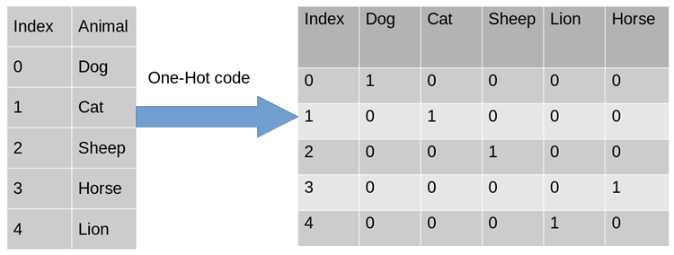
#Why can I use One-Hot Encoding?
使用one-hot编码,将离散特征的取值扩展到了欧式空间,离散特征的某个取值就对应欧式空间的某个点。在回归,分类,聚类等机器学习算法中,特征之间距离的计算或相似度的计算是非常重要的,而我们常用的距离或相似度的计算都是在欧式空间的相似度计算,计算余弦相似性,也是基于的欧式空间。
使用One-Hot编码对离散型特征进行处理可以使得特征之间的距离计算更加准确。比如,有一个离散型特征,代表工作类型,该离散型特征,共有三个取值,不使用one-hot编码,计算出来的特征的距离是不合理。那如果使用one-hot编码,显得更合理。
独热编码优缺点
优点:独热编码解决了分类器不好处理属性数据的问题,在一定程度上也起到了扩充特征的作用。它的值只有0和1,不同的类型存储在垂直的空间。
缺点:当类别的数量很多时,特征空间会变得非常大。在这种情况下,一般可以用PCA(主成分分析)来减少维度。在实际应用中,One-Hot Encoding与PCA结合的方法也非常实用。
One-Hot Encoding的使用场景
独热编码用来解决类别型数据的离散值问题。将离散型特征进行one-hot编码的作用,是为了让距离计算更合理,但如果特征是离散的,并且不用one-hot编码就可以很合理的计算出距离,那么就没必要进行one-hot编码,比如,该离散特征共有1000个取值,我们分成两组,分别是400和600,两个小组之间的距离有合适的定义,组内的距离也有合适的定义,那就没必要用one-hot 编码。
树结构方法,如随机森林、Bagging和Boosting等,在特征处理方面不需要进行标准化操作。对于决策树来说,one-hot的本质是增加树的深度,决策树是没有特征大小的概念的,只有特征处于他分布的哪一部分的概念。
基于Scikit-learn 的one hot encoding
LabelBinarizer:将对应的数据转换为二进制型,类似于onehot编码,这里有几点不同:
可以处理数值型和类别型数据
输入必须为1D数组
可以自己设置正类和父类的表示方式
from sklearn.preprocessing import LabelBinarizer lb = LabelBinarizer() city_list = ["paris", "paris", "tokyo", "amsterdam"] lb.fit(city_list) print(lb.classes_) # 输出为:['amsterdam' 'paris' 'tokyo'] city_list_le = lb.transform(city_list) # 进行Encode print(city_list_le) # 输出为: # [[0 1 0] # [0 1 0] # [0 0 1] # [1 0 0]] city_list_new = lb.inverse_transform(city_list_le) # 进行decode print(city_list_new) # 输出为:['paris' 'paris' 'tokyo' 'amsterdam']
OneHotEncoder只能对数值型数据进行处理,需要先将文本转化为数值(Label encoding)后才能使用,只接受2D数组:
import pandas as pd from sklearn.preprocessing import LabelEncoder from sklearn.preprocessing import OneHotEncoder def LabelOneHotEncoder(data, categorical_features): d_num = np.array([]) for f in data.columns: if f in categorical_features: le, ohe = LabelEncoder(), OneHotEncoder() data[f] = le.fit_transform(data[f]) if len(d_num) == 0: d_num = np.array(ohe.fit_transform(data[[f]])) else: d_num = np.hstack((d_num, ohe.fit_transform(data[[f]]).A)) else: if len(d_num) == 0: d_num = np.array(data[[f]]) else: d_num = np.hstack((d_num, data[[f]])) return d_num df = pd.DataFrame([ ['green', 'Chevrolet', 2017], ['blue', 'BMW', 2015], ['yellow', 'Lexus', 2018], ]) df.columns = ['color', 'make', 'year'] df_new = LabelOneHotEncoder(df, ['color', 'make', 'year'])
基于Pandas的one hot encoding
其实如果我们跳出 scikit-learn, 在 pandas 中可以很好地解决这个问题,用 pandas 自带的get_dummies函数即可
import pandas as pd df = pd.DataFrame([ ['green', 'Chevrolet', 2017], ['blue', 'BMW', 2015], ['yellow', 'Lexus', 2018], ]) df.columns = ['color', 'make', 'year'] df_processed = pd.get_dummies(df, prefix_sep="_", columns=df.columns[:-1]) print(df_processed)
get_dummies的优势在于:
本身就是 pandas 的模块,所以对 DataFrame 类型兼容很好
不管你列是数值型还是字符串型,都可以进行二值化编码
能够根据指令,自动生成二值化编码后的变量名
get_dummies虽然有这么多优点,但毕竟不是 sklearn 里的transformer类型,所以得到的结果得手动输入到 sklearn 里的相应模块,也无法像 sklearn 的transformer一样可以输入到pipeline中进行流程化地机器学习过程。
将类别特征替换为训练集中的计数(一般是根据训练集来进行计数,属于统计编码的一种,统计编码,就是用类别的统计特征来代替原始类别,比如类别A在训练集中出现了100次则编码为100)。这个方法对离群值很敏感,所以结果可以归一化或者转换一下(例如使用对数变换)。未知类别可以替换为1。
频数编码使用频次替换类别。有些变量的频次可能是一样的,这将导致碰撞。尽管可能性不是非常大,没法说这是否会导致模型退化,不过原则上我们不希望出现这种情况。
import pandas as pd data_count = data.groupby('城市')['城市'].agg({'频数':'size'}).reset_index() data = pd.merge(data, data_count, on = '城市', how = 'left')
目标编码(target encoding),亦称均值编码(mean encoding)、似然编码(likelihood encoding)、效应编码(impact encoding),是一种能够对高基数(high cardinality)自变量进行编码的方法 (Micci-Barreca 2001) 。
如果某一个特征是定性的(categorical),而这个特征的可能值非常多(高基数),那么目标编码(Target encoding)是一种高效的编码方式。在实际应用中,这类特征工程能极大提升模型的性能。
一般情况下,针对定性特征,我们只需要使用sklearn的OneHotEncoder或LabelEncoder进行编码。
LabelEncoder can receive irregular feature columns and convert them into integer values from 0 to n-1 (assuming there are n different categories in total); OneHotEncoder can produce an m*n through dummy encoding A sparse matrix (assuming there are m rows of data in total, whether the specific output matrix format is sparse can be controlled by the sparse parameter).
"Cardinality" of a qualitative characteristic refers to the total number of distinct possible values that the characteristic can take.. In the face of high cardinality qualitative characteristics, these data preprocessing methods often fail to achieve satisfactory results.
Examples of high-cardinality qualitative features: IP address, email domain name, city name, home address, street, product number.
Main reason:
LabelEncoder encodes high-cardinality qualitative features. Although only one column is required, each natural number has different significance. Linearly inseparable with respect to y. Using a simple model is prone to underfitting and cannot fully capture the differences between different categories; using a complex model is prone to overfitting in other places.
OneHotEncoder encodes high-cardinality qualitative features, which will inevitably produce a sparse matrix with tens of thousands of columns, which will easily consume a lot of memory and training time, unless the algorithm itself has relevant optimizations (for example: SVM).
If the cardinality of a certain categorical feature is relatively low (low-cardinality features), that is, the number of elements in the set composed of all values of the feature after deduplication is relatively small, generally use One- The hot encoding method converts features into numerical types. One-hot encoding can be completed during data preprocessing or during model training. From the perspective of training time, the latter method is more efficient. CatBoost also uses the latter method for categorical features with low cardinality. kind of realization.
Obviously, among high cardinality features, such as user ID, this encoding method will generate a large number of new features, causing a dimensionality disaster. A compromise method is to group the categories into a limited number of groups and then perform One-hot encoding. A commonly used method is to group according to target variable statistics (Target Statistics, hereinafter referred to as TS), which is used to estimate the expected value of the target variable for each category. Some people even directly use TS as a new numerical variable to replace the original categorical variable. Importantly, by setting the threshold for TS numerical features, based on logarithmic loss, Gini coefficient or mean square error, we can obtain the optimal one among all possible divisions that divide the category into two for the training set. In LightGBM, categorical features are represented by Gradient Statistics (GS) at each step of gradient boosting. Although it provides important information for tree building, this method has the following two disadvantages:
Increases the calculation time because it requires each categorical feature at each step of the iteration. GS needs to be calculated
Increases storage requirements. For a categorical variable, it is necessary to store the category of each node separated each time
In order to overcome these shortcomings, LightGBM classifies all long-tail categories into one category at the cost of losing some information. The author claims that this method is much better than One-hot encoding when processing high-cardinality category features. Using TS features, only one number per category is calculated and stored. Therefore, using TS as a new numerical feature for processing categorical features is the most effective and can minimize information loss. TS is also widely used in click prediction tasks. The category features in this scenario include users, regions, advertisements, advertisement publishers, etc. In the following discussion, we will focus on TS and leave One-hot encoding and GS aside for now.
The following is the calculation formula:
where n represents the number of values of a certain feature,
represents the value of a certain feature The lower number is the number of positive Labels. mdl is a minimum threshold. Feature categories with a sample number less than this value will be ignored. Prior is the mean value of the Label. Note that if you are dealing with a regression problem, it can be processed into the average/max of the label value under the corresponding feature. For k classification problems, corresponding k-1 features will be generated.
This method is also easy to cause over-fitting. The following methods are used to prevent over-fitting:
Increase the size of the regular term a
Add noise to this column of the training set
Use cross-validation
The target encoding is supervised The coding method, if used properly, can effectively improve the accuracy of the prediction model (Pargent, Bischl, and Thomas 2019); and the key to this is to introduce regularization in the coding process to avoid over-fitting problems.
For example, category A corresponds to 200 tags 1, 300 tags 2, and 500 tags 3. It can be coded as: 2/10, 3/10, 3/6. The most important thing in the middle is how to avoid overfitting (the original target encoding directly encodes all training set data and labels, which will cause the obtained encoding results to be too dependent on the training set). A common solution is to use 2 levels of Cross-validation finds the target mean. The idea is as follows:
把train data划分为20-folds (举例:infold: fold #2-20, out of fold: fold #1)
计算 10-folds的 inner out of folds值 (举例:使用inner_infold #2-10 的target的均值,来作为inner_oof #1的预测值)
对10个inner out of folds 值取平均,得到 inner_oof_mean
将每一个 infold (fold #2-20) 再次划分为10-folds (举例:inner_infold: fold #2-10, Inner_oof: fold #1)
计算oof_mean (举例:使用 infold #2-20的inner_oof_mean 来预测 out of fold #1的oof_mean
将train data 的 oof_mean 映射到test data完成编码
比如划分为10折,每次对9折进行标签编码然后用得到的标签编码模型预测第10折的特征得到结果,其实就是常说的均值编码。
目标编码尝试对分类特征中每个级别的目标总体平均值进行测量。当数据量较少时,每个级别的数据量减少意味着估计的均值与真实均值之间的差距增加,方差也会更大。
from category_encoders import TargetEncoder import pandas as pd from sklearn.datasets import load_boston # prepare some data bunch = load_boston() y_train = bunch.target[0:250] y_test = bunch.target[250:506] X_train = pd.DataFrame(bunch.data[0:250], columns=bunch.feature_names) X_test = pd.DataFrame(bunch.data[250:506], columns=bunch.feature_names) # use target encoding to encode two categorical features enc = TargetEncoder(cols=['CHAS', 'RAD']) # transform the datasets training_numeric_dataset = enc.fit_transform(X_train, y_train) testing_numeric_dataset = enc.transform(X_test)
Kaggle竞赛Avito Demand Prediction Challenge 第14名的solution分享:14th Place Solution: The Almost Golden Defenders。和target encoding 一样,beta target encoding 也采用 target mean value (among each category) 来给categorical feature做编码。不同之处在于,为了进一步减少target variable leak,beta target encoding发生在在5-fold CV内部,而不是在5-fold CV之前:
把train data划分为5-folds (5-fold cross validation)
target encoding based on infold data
train model
get out of fold prediction
同时beta target encoding 加入了smoothing term,用 bayesian mean 来代替mean。Bayesian mean (Bayesian average) 的思路:某一个category如果数据量较少(
另外,对于target encoding和beta target encoding,不一定要用target mean (or bayesian mean),也可以用其他的统计值包括 medium, frqequency, mode, variance, skewness, and kurtosis — 或任何与target有correlation的统计值。
# train -> training dataframe # test -> test dataframe # N_min -> smoothing term, minimum sample size, if sample size is less than N_min, add up to N_min # target_col -> target column # cat_cols -> categorical colums # Step 1: fill NA in train and test dataframe # Step 2: 5-fold CV (beta target encoding within each fold) kf = KFold(n_splits=5, shuffle=True, random_state=0) for i, (dev_index, val_index) in enumerate(kf.split(train.index.values)): # split data into dev set and validation set dev = train.loc[dev_index].reset_index(drop=True) val = train.loc[val_index].reset_index(drop=True) feature_cols = [] for var_name in cat_cols: feature_name = f'{var_name}_mean' feature_cols.append(feature_name) prior_mean = np.mean(dev[target_col]) stats = dev[[target_col, var_name]].groupby(var_name).agg(['sum', 'count'])[target_col].reset_index() ### beta target encoding by Bayesian average for dev set df_stats = pd.merge(dev[[var_name]], stats, how='left') df_stats['sum'].fillna(value = prior_mean, inplace = True) df_stats['count'].fillna(value = 1.0, inplace = True) N_prior = np.maximum(N_min - df_stats['count'].values, 0) # prior parameters dev[feature_name] = (prior_mean * N_prior + df_stats['sum']) / (N_prior + df_stats['count']) # Bayesian mean ### beta target encoding by Bayesian average for val set df_stats = pd.merge(val[[var_name]], stats, how='left') df_stats['sum'].fillna(value = prior_mean, inplace = True) df_stats['count'].fillna(value = 1.0, inplace = True) N_prior = np.maximum(N_min - df_stats['count'].values, 0) # prior parameters val[feature_name] = (prior_mean * N_prior + df_stats['sum']) / (N_prior + df_stats['count']) # Bayesian mean ### beta target encoding by Bayesian average for test set df_stats = pd.merge(test[[var_name]], stats, how='left') df_stats['sum'].fillna(value = prior_mean, inplace = True) df_stats['count'].fillna(value = 1.0, inplace = True) N_prior = np.maximum(N_min - df_stats['count'].values, 0) # prior parameters test[feature_name] = (prior_mean * N_prior + df_stats['sum']) / (N_prior + df_stats['count']) # Bayesian mean # Bayesian mean is equivalent to adding N_prior data points of value prior_mean to the data set. del df_stats, stats # Step 3: train model (K-fold CV), get oof predictio
M-Estimate Encoding 相当于 一个简化版的Target Encoding:
其中????+代表所有正Label的个数,m是一个调参的参数,m越大过拟合的程度就会越小,同样的在处理连续值时????+可以换成label的求和,????+换成所有label的求和。
一种基于目标的算法是 James-Stein 编码。算法的思想很简单,对于特征的每个取值 k 可以根据下面的公式获得:
其中B由以下公式估计:
但是它有一个要求是target必须符合正态分布,这对于分类问题是不可能的,因此可以把y先转化成概率的形式。在实际操作中,可以使用网格搜索方法来选择一个较优的B值。
Weight Of Evidence 同样是基于target的方法。
使用WOE作为变量,第i类的WOE等于:
WOE特别合适逻辑回归,因为Logit=log(odds)。WOE编码的变量被编码为统一的维度(是一个被标准化过的值),变量之间直接比较系数即可。
这个方法类似于SUM的方法,只是在计算训练集每个样本的特征值转换时都要把该样本排除(消除特征某取值下样本太少导致的严重过拟合),在计算测试集每个样本特征值转换时与SUM相同。可见以下公式:
使用二进制编码对每一类进行编号,使用具有log2N维的向量对N类进行编码。以 (0,0) 为例,它表示第一类,而 (0,1) 表示第二类,(1,0) 表示第三类,(1,1) 则表示第四类
类似于One-hot encoding,但是通过hash函数映射到一个低维空间,并且使得两个类对应向量的空间距离基本保持一致。使用低维空间来降低了表示向量的维度。
特征哈希可能会导致要素之间发生冲突。一个哈希编码的好处是不需要指定或维护原变量与新变量之间的映射关系。因此,哈希编码器的大小及复杂程度不随数据类别的增多而增多。
和WOE相似,只是去掉了log,即:
Performs sum encoding on a certain feature by comparing the mean value of the label (or other related variables) under the feature value with the mean value of the overall label differences between them to encode features. If the details are not done well, this method is very prone to overfitting, so it needs to be combined with the leave-one-out method or five-fold cross-validation to encode features. There are also methods to add a penalty term based on the variance to prevent overfitting.
Helmert encoding is commonly used in econometrics. After Helmert encoding (each value in the categorical feature corresponds to a row in the Helmert matrix), the encoded variable coefficients in the linear model can reflect the mean value of the dependent variable given a certain category value of the category variable. The difference between the means of the dependent variable given the values for the other categories in that category.
Helmet encoding is the most widely used encoding method after One-Hot Encoding and Sum Encoder. Different from Sum Encoder, it compares the corresponding label (or other related variables) under a certain feature value. ) is compared to the mean of its previous features, rather than to the mean of all features. This feature is also prone to overfitting.
For categorical variables whose number of possible values is larger than the one-hot maximum, CatBoost uses a very effective encoding method, which is similar to mean encoding. But it can reduce overfitting. Its specific implementation method is as follows:
Randomly sort the input sample set and generate multiple groups of random arrangements.
Convert floating point or attribute value tags to integers.
Convert all classification feature value results into numerical results according to the following formula.
Among them, CountInClass indicates how many samples have a mark value of 1 in the current classification feature value; Prior is the initial value of the molecule, determined according to the initial parameters. TotalCount represents the number of all samples with the same classification feature value as the current sample, including the current sample itself.
Summary of CatBoost processing Categorical features:
First, they will calculate statistics of some data. Calculate the frequency of occurrence of a category, add hyperparameters, and generate new numerical features. This strategy requires that data with the same label cannot be arranged together (that is, all 0s first and then all 1s), and the data set needs to be scrambled before training.
Second, use different permutations of the data (actually 4). Before building the tree each round, a round of dice is thrown to decide which arrangement to use to build the tree.
The third point is to consider trying different combinations of categorical features. For example, color and type can be combined to form a feature similar to blue dog. When the number of categorical features that need to be combined increases, catboost only considers some combinations. When selecting the first node, only one feature, such as A, is considered. When generating the second node, consider the combination of A and any categorical feature and choose the best one. In this way, a greedy algorithm is used to generate combinations.
Fourth, unless the dimension is very small like gender, it is not recommended to generate one-hot vectors by yourself. It is best to leave it to the algorithm.
The above is the detailed content of What are the methods for processing categorical features in Python machine learning?. For more information, please follow other related articles on the PHP Chinese website!


![[Web front-end] Node.js quick start](https://img.php.cn/upload/course/000/000/067/662b5d34ba7c0227.png)


