The so-called linear least squares method can be understood as a continuation of solving equations. The difference is that when the unknown quantity is far smaller than the number of equations, an unsolvable problem will be obtained. The essence of the least squares method is to assign values to unknown numbers while ensuring the minimum error.
The least squares method is a very classic algorithm, and we have been exposed to this name in high school. It is an extremely commonly used algorithm. I have previously written about the principle of linear least squares and implemented it in Python: least squares and its Python implementation; and how to call nonlinear least squares in scipy: nonlinear least squares(Supplementary content at the end of the article);There is also the least squares method of sparse matrices: sparse matrix least squares method.
The following describes the linear least squares method implemented in numpy and scipy, and compares the speed of the two.
numpy implementation
The least squares method is implemented in numpy, that is, lstsq(a,b) is used to solve x similar to a@x=b, where a is M× N matrix; then when b is a vector of M rows, it is just equivalent to solving a system of linear equations. For a system of equations like Ax=b, if A is a full-rank simulation, it can be expressed as x=A−1b, otherwise it can be expressed as x=(ATA)−1ATb.
When b is a matrix of M×K, then for each column, a set of x will be calculated.
There are 4 return values, which are the x obtained by fitting, the fitting error, the rank of matrix a, and the single-valued form of matrix a.
import numpy as np
np.random.seed(42)
M = np.random.rand(4,4)
x = np.arange(4)
y = M@x
xhat = np.linalg.lstsq(M,y)
print(xhat[0])
#[0. 1. 2. 3.]
scipy package
scipy.linalg also provides the least squares function. The function name is also lstsq, and its parameter list is
where a, b is Ax= b. Both provide overridable switches. Setting them to True can save running time. In addition, the function also supports finiteness checking, which is an option that many functions in linalg have. Its return value is the same as the least squares function in numpy.
cond is a floating point parameter, indicating the singular value threshold. When the singular value is less than cond, it will be discarded.
lapack_driver is a string option, indicating which algorithm engine in LAPACK is selected, optionally 'gelsd', 'gelsy', 'gelss'.
Finally, make a speed comparison between the two sets of least squares functions
from timeit import timeit
N = 100
A = np.random.rand(N,N)
b = np.arange(N)

timeit(lambda:np.linalg.lstsq(A, b), number=10)
# 0.015487500000745058
timeit(lambda:sl.lstsq(A, b), number=10)
# 0.011151800004881807
This time, the two are not too far apart The difference is that even if the matrix dimension is enlarged to 500, the two are about the same.
N = 500
A = np.random.rand(N,N)
b = np.arange(N)

timeit(lambda:np.linalg.lstsq(A, b), number=10)
0.389679799991427
timeit(lambda:sl.lstsq(A, b), number=10)
0.35642060000100173
Supplement
Python calls the nonlinear least squares method
Introduction and constructor
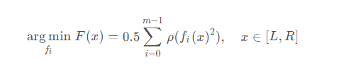
In In scipy, the purpose of the nonlinear least squares method is to find a set of functions that minimize the sum of squares of the error function, which can be expressed as the following formula
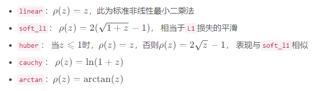
where ρ represents the loss function , can be understood as a preprocessing of fi(x).
scipy.optimize encapsulates the nonlinear least squares function least_squares, which is defined as
Among them, func and x0 are required parameters, func is the function to be solved, and x0 is the function input The initial value of , there is no default value for these two parameters, they are parameters that must be entered.
bound is the solution interval, the default is (−∞,∞). When verbose is 1, there will be a termination output. When verbose is 2, more information during the operation will be printed. In addition, the following parameters are used to control the error, which is relatively simple.
import numpy as np
from scipy.optimize import least_squares

def test(xs):
    _sum = 0.0
    for i in range(len(xs)):
        _sum = _sum + (1-np.cos((xs[i]*i)/5)*(i+1))
    return _sum

x0 = np.random.rand(5)
ret = least_squares(test, x0)
msg = f"最小值" + ", ".join([f"{x:.4f}" for x in ret.x])
msg += f"\nf(x)={ret.fun[0]:.4f}"
print(msg)
'''
最小值0.9557, 0.5371, 1.5714, 1.6931, 5.2294
f(x)=0.0000
'''
The above is the detailed content of How to call and implement the least squares method in Python. For more information, please follow other related articles on the PHP Chinese website!
Statement of this Website
The content of this article is voluntarily contributed by netizens, and the copyright belongs to the original author. This site does not assume corresponding legal responsibility. If you find any content suspected of plagiarism or infringement, please contact admin@php.cn
First, define a ContactForm form containing name, mailbox and message fields; 2. In the view, the form submission is processed by judging the POST request, and after verification is passed, cleaned_data is obtained and the response is returned, otherwise the empty form will be rendered; 3. In the template, use {{form.as_p}} to render the field and add {%csrf_token%} to prevent CSRF attacks; 4. Configure URL routing to point /contact/ to the contact_view view; use ModelForm to directly associate the model to achieve data storage. DjangoForms implements integrated processing of data verification, HTML rendering and error prompts, which is suitable for rapid development of safe form functions.
Install pyodbc: Use the pipinstallpyodbc command to install the library; 2. Connect SQLServer: Use the connection string containing DRIVER, SERVER, DATABASE, UID/PWD or Trusted_Connection through the pyodbc.connect() method, and support SQL authentication or Windows authentication respectively; 3. Check the installed driver: Run pyodbc.drivers() and filter the driver name containing 'SQLServer' to ensure that the correct driver name is used such as 'ODBCDriver17 for SQLServer'; 4. Key parameters of the connection string
shutil.rmtree() is a function in Python that recursively deletes the entire directory tree. It can delete specified folders and all contents. 1. Basic usage: Use shutil.rmtree(path) to delete the directory, and you need to handle FileNotFoundError, PermissionError and other exceptions. 2. Practical application: You can clear folders containing subdirectories and files in one click, such as temporary data or cached directories. 3. Notes: The deletion operation is not restored; FileNotFoundError is thrown when the path does not exist; it may fail due to permissions or file occupation. 4. Optional parameters: Errors can be ignored by ignore_errors=True
iter() is used to obtain the iterator object, and next() is used to obtain the next element; 1. Use iterator() to convert iterable objects such as lists into iterators; 2. Call next() to obtain elements one by one, and trigger StopIteration exception when the elements are exhausted; 3. Use next(iterator, default) to avoid exceptions; 4. Custom iterators need to implement the __iter__() and __next__() methods to control iteration logic; using default values is a common way to safe traversal, and the entire mechanism is concise and practical.
Introduction to Statistical Arbitrage Statistical Arbitrage is a trading method that captures price mismatch in the financial market based on mathematical models. Its core philosophy stems from mean regression, that is, asset prices may deviate from long-term trends in the short term, but will eventually return to their historical average. Traders use statistical methods to analyze the correlation between assets and look for portfolios that usually change synchronously. When the price relationship of these assets is abnormally deviated, arbitrage opportunities arise. In the cryptocurrency market, statistical arbitrage is particularly prevalent, mainly due to the inefficiency and drastic fluctuations of the market itself. Unlike traditional financial markets, cryptocurrencies operate around the clock and their prices are highly susceptible to breaking news, social media sentiment and technology upgrades. This constant price fluctuation frequently creates pricing bias and provides arbitrageurs with
Use psycopg2.pool.SimpleConnectionPool to effectively manage database connections and avoid the performance overhead caused by frequent connection creation and destruction. 1. When creating a connection pool, specify the minimum and maximum number of connections and database connection parameters to ensure that the connection pool is initialized successfully; 2. Get the connection through getconn(), and use putconn() to return the connection to the pool after executing the database operation. Constantly call conn.close() is prohibited; 3. SimpleConnectionPool is thread-safe and is suitable for multi-threaded environments; 4. It is recommended to implement a context manager in combination with context manager to ensure that the connection can be returned correctly when exceptions are noted;
Install the corresponding database driver; 2. Use connect() to connect to the database; 3. Create a cursor object; 4. Use execute() or executemany() to execute SQL and use parameterized query to prevent injection; 5. Use fetchall(), etc. to obtain results; 6. Commit() is required after modification; 7. Finally, close the connection or use a context manager to automatically handle it; the complete process ensures that SQL operations are safe and efficient.


 Backend Development