How to draw a double pie chart with connecting lines in Python

1. Import the required libraries

import matplotlib.pyplot as plt
import numpy as np
from matplotlib.patches import ConnectionPatch
from matplotlib import cm

The ConnectionPatch class in the matplotlib.patches module can be used to draw the connection between two subplots. In visualizations such as a double pie chart, you can use this class to draw a connection between two subgraphs to express the relationship between them. This class provides many parameters and methods that can be used to control properties such as the style and position of the connection.

ConnectionPatch is used to add connections in Matplotlib. Its main parameters are as follows:

• xyA: the starting point of the connection line;

• xyB: The end point of the connecting line;

• coordsA: The coordinate system of the starting point, the default is data;

• coordsB: End The coordinate system of the point, the default is data;

• axesA: the Axes object where the starting point is located;

• axesB: the Axes object where the end point is located ;

• color: the color of the connecting line;

• linewidth: the line width of the connecting line;

• linestyle: The line style of the connecting line.

Commonly used methods of ConnectionPatch include:

• set_color: Set the color of the connection line;

• set_linewidth: Set the line width of the connecting line;

• set_linestyle: Set the line style of the connecting line.

cm is the color mapping module of Matplotlib. It provides a series of color schemes, including single tone, segmented coloring and continuous gradient coloring, etc., which can Better meet the needs of data visualization.

2. Prepare data

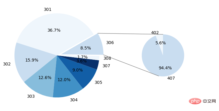
# 大饼图数据
labels = ['301', '302', '303', '304', '305', '307', '308', '306']
size = [219324, 94739, 75146, 71831, 54051, 21458, 9990, 50843]
# 大饼图分裂距离
explode = (0, 0, 0, 0, 0, 0, 0, 0.1)
# 小饼图数据
labels2 = ['402', '407']
size2 = [12255, 207069]
width = 0.2

This code is used to define the data of the big pie chart and the small pie chart, and set the splitting distance of the big pie chart and the width of the small pie chart.

The specific explanation is as follows:

• labels: Define the label of each split block of the pie chart, that is, which area it represents.

• size: Define the size of each split block of the pie chart, which means the number or proportion of each area.

• explode: Define the distance between each split block of the big pie chart and the center of the pie, that is, whether the split block needs to pop up. Here it is set to not pop up.

• labels2: Define the label of each split block of the small pie chart, that is, which area it represents.

• size2: Define the size of each split block of the small pie chart, which means the number or proportion of each area.

• width: Define the width of the small pie chart, here set to 0.2.

3. Draw a double pie chart

3.1 Create canvas and subgraph objects

fig = plt.figure(figsize=(9, 5))
ax1 = fig.add_subplot(121)
ax2 = fig.add_subplot(122)

This part of the code creates a size (9, 5) Canvas fig, and added two sub-figures ax1 and ax2 on the canvas.

Among them, fig.add_subplot(121) means dividing the canvas into subplots with 1 row and 2 columns, and select the first subplot (i.e. the subplot on the left); fig .add_subplot(122) means selecting the second subplot (that is, the subplot on the right). The numbering rule of the subgraph is similar to the array index. The row number increases from 1 from top to bottom, and the column number increases from 1 from left to right. For example, (1, 1) represents the subgraph of the first row and first column, ( 1, 2) represents the subgraph of the first row and second column. Here 121 and 122 represent the first and second subgraphs of the first row respectively.

3.2 Drawing a big pie chart

ax1.pie(size,
        autopct='%1.1f%%',
        startangle=30,
        labels=labels,
        colors=cm.Blues(range(10, 300, 50)),
        explode=explode)

This code is used to draw a pie chart in the first subgraph (ax1). The meaning of the specific parameters is as follows:

• size: Pie chart data, indicating the size of each pie chart block.

• autopct: The data label format of the pie chart block, "%1.1f%%" means retaining one decimal place and adding a percent sign.

• startangle: The starting angle of the pie chart block, 30 degrees is the starting point, rotate clockwise.

• labels: Labels of pie chart blocks, corresponding to size.

• colors: The color of the pie chart block, using the cm.Blues() function to generate a color list.

• explode: The splitting distance of the pie chart block, indicating whether it is separated from the center of the pie chart. For example (0, 0, 0, 0, 0, 0, 0, 0.1) means that the last pie piece is 0.1 radii away from the center.

You can adjust these parameters and other parameters of the pie chart as needed to get the desired effect.

3.3 Drawing a small pie chart

ax2.pie(size2,
        autopct='%1.1f%%',
        startangle=90,
        labels=labels2,
        colors=cm.Blues(range(10, 300, 50)),
        radius=0.5,
        shadow=False)

This code is used to draw the second small pie chart. The specific parameter meanings are as follows:

• size2: the data of the small pie chart, that is, [12255, 207069];

• autopct: format wedge shape The data label of the block, ‘%1.1f%%’ means keeping one decimal place and adding a percent sign after it;

• ##startangle: the starting angle of the small pie chart , expressed in degrees, here it is set to 90 degrees, that is, starting from the vertical direction;

• labels2: The labels of the small pie chart, that is, [‘402’, ‘407’] ;

• colors: Specify the color, here use cm.Blues function to generate a set of blue series colors;

• radius: small pie chart Radius, set to 0.5 here;

• shadow: whether to add a shadow, set to False here.

在这段代码中，我们创建了一个名为 ax2 的子区域对象，并使用 pie 方法绘制了一个小饼图，将 size2 中的数据作为输入数据。其他参数指定了锲形块的格式、颜色、标签等属性，进一步定制了图形的样式。

3.4 连接线1，连接大饼图的上边缘和小饼图的饼块

theta1, theta2 = ax1.patches[-1].theta1, ax1.patches[-1].theta2
center, r = ax1.patches[-1].center, ax1.patches[-1].r
x = r * np.cos(np.pi / 180 * theta2) + center[0]
y = np.sin(np.pi / 180 * theta2) + center[1]
con1 = ConnectionPatch(xyA=(0, 0.5),
                       xyB=(x, y),
                       coordsA=ax2.transData,
                       coordsB=ax1.transData,
                       axesA=ax2, axesB=ax1)

这部分代码是用来计算连接两个饼图的连接线的起点和终点位置，并创建一个 ConnectionPatch 对象用于绘制连接线。

• theta1 和 theta2 分别表示饼图上最后一个扇形的起始角度和终止角度。

• center 表示饼图中最后一个扇形的中心点位置。

• r 表示饼图的半径。

• x 和 y 表示连接线的终点坐标，其中 x 通过利用三角函数计算出来。

接下来，ConnectionPatch 的参数解释：

• xyA 表示连接线的起点位置，这里设为 (0, 0.5) 表示在小饼图上以它的左边中间位置为起点。

• xyB 表示连接线的终点位置，这里为 (x, y) 表示在大饼图上以计算得到的 x 和 y 为终点位置。

• coordsA 和 coordsB 表示起点和终点所在的坐标系，这里分别为小饼图和大饼图的坐标系。

• axesA 和 axesB 分别表示起点和终点所在的子图对象，这里分别为小饼图和大饼图的子图对象，即 ax2 和 ax1。

3.5 连接线2，连接大饼图的下边缘和小饼图的饼块

x = r * np.cos(np.pi / 180 * theta1) + center[0]
y = np.sin(np.pi / 180 * theta1) + center[1]
con2 = ConnectionPatch(xyA=(-0.1, -0.49),
                       xyB=(x, y),
                       coordsA='data',
                       coordsB='data',
                       axesA=ax2, axesB=ax1)

这段代码用于创建连接线的第二个对象con2。具体解释如下：

• x 和 y 分别代表了连接线从小饼图中(-0.1,-0.49)这个点出发，到大饼图中theta1角度对应的点的终点坐标。其中，theta1是通过访问ax1.patches[-1].theta1获得的。

• coordsA 和 coordsB 表示终点和起点坐标的坐标系类型。这里都是 ‘data’ 表示使用数据坐标系，即默认的 x 和 y 坐标值。

• axesA 和 axesB 表示终点和起点所在的子图对象。其中，axesA 为小饼图，axesB 为大饼图。

• 这里使用ConnectionPatch函数创建连接线对象。

3.6 添加连接线

for con in [con1, con2]:
    con.set_color('gray')
    ax2.add_artist(con)
    con.set_linewidth(1)

这段代码用于设置连接线的颜色和粗细，并将连接线添加到小饼图的坐标系上。具体来说，循环遍历连接线对象列表 [con1, con2]，并依次对每个连接线进行以下操作：

• 调用 set_color() 方法设置连接线的颜色为灰色。

• 调用 ax2.add_artist() 方法将连接线添加到小饼图的坐标系上。

• 调用 set_linewidth() 方法设置连接线的宽度为 1。

3.7 调整子图布局

fig.subplots_adjust(wspace=0)
plt.show()

这行代码调整了子图之间的水平间距，将间距设置为0，即将子图紧密排列。wspace参数表示子图之间的宽度间距。具体来说，这行代码将第一个子图和第二个子图之间的间距设置为0，使它们之间没有空隙。

四、源代码

import matplotlib.pyplot as plt
import numpy as np
from matplotlib.patches import ConnectionPatch
from matplotlib import cm
# 大饼图数据
labels = ['301', '302', '303', '304', '305', '307', '308', '306']
size = [219324, 94739, 75146, 71831, 54051, 21458, 9990, 50843]
# 大饼图分裂距离
explode = (0, 0, 0, 0, 0, 0, 0, 0.1)
# 小饼图数据
labels2 = ['402', '407']
size2 = [12255, 207069]
width = 0.2
# 创建画布和子图对象
fig = plt.figure(figsize=(9, 5))
ax1 = fig.add_subplot(121)
ax2 = fig.add_subplot(122)
# 绘制大饼图
ax1.pie(size,
        autopct='%1.1f%%',
        startangle=30,
        labels=labels,
        colors=cm.Blues(range(10, 300, 50)),
        explode=explode)
# 绘制小饼图
ax2.pie(size2,
        autopct='%1.1f%%',
        startangle=90,
        labels=labels2,
        colors=cm.Blues(range(10, 300, 50)),
        radius=0.5,
        shadow=False)
# 连接线1，连接大饼图的上边缘和小饼图的饼块
theta1, theta2 = ax1.patches[-1].theta1, ax1.patches[-1].theta2
center, r = ax1.patches[-1].center, ax1.patches[-1].r
x = r * np.cos(np.pi / 180 * theta2) + center[0]
y = np.sin(np.pi / 180 * theta2) + center[1]
con1 = ConnectionPatch(xyA=(0, 0.5),
                       xyB=(x, y),
                       coordsA=ax2.transData,
                       coordsB=ax1.transData,
                       axesA=ax2, axesB=ax1)
# 连接线2，连接大饼图的下边缘和小饼图的饼块
x = r * np.cos(np.pi / 180 * theta1) + center[0]
y = np.sin(np.pi / 180 * theta1) + center[1]
con2 = ConnectionPatch(xyA=(-0.1, -0.49),
                       xyB=(x, y),
                       coordsA='data',
                       coordsB='data',
                       axesA=ax2, axesB=ax1)
# 添加连接线
for con in [con1, con2]:
    con.set_color('gray')
    ax2.add_artist(con)
    con.set_linewidth(1)
# 调整子图布局
fig.subplots_adjust(wspace=0)
# 显示图像
plt.show()

可视化结果为：

The above is the detailed content of How to draw a double pie chart with connecting lines in Python. For more information, please follow other related articles on the PHP Chinese website!