Comparison of common dimensionality reduction technologies: feasibility analysis of reducing data dimensions while maintaining information integrity

This article will compare the effectiveness of various dimensionality reduction techniques on tabular data in machine learning tasks. We apply dimensionality reduction methods to the dataset and evaluate their effectiveness through regression and classification analyses. We apply dimensionality reduction methods to various datasets obtained from UCI related to different domains. A total of 15 datasets were selected, 7 of which will be used for regression and 8 for classification.

To make this article easy to read and understand, only the preprocessing and analysis of one dataset is shown. The experiment starts by loading the dataset. The data set is split into training and test sets and then normalized to have a mean of 0 and a standard deviation of 1.

Dimensionality reduction techniques are then applied to the training data and the test set is transformed for dimensionality reduction using the same parameters. For regression, principal component analysis (PCA) and singular value decomposition (SVD) are used for dimensionality reduction. On the other hand, for classification, linear discriminant analysis (LDA) is used.

After dimensionality reduction, multiple machine learning models are trained Tests were conducted and the performance of different models was compared on different datasets obtained through different dimensionality reduction methods.

Let us start the process by loading the first dataset,

import pandas as pd ## for data manipulation df = pd.read_excel(r'RegressionAirQualityUCI.xlsx') print(df.shape) df.head()

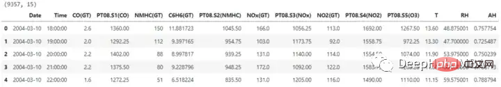
The dataset contains 15 columns, One of them is the need to predict labels. Before continuing with dimensionality reduction, the date and time columns are also removed.

X = df.drop(['CO(GT)', 'Date', 'Time'], axis=1) y = df['CO(GT)'] X.shape, y.shape #Output: ((9357, 12), (9357,))

For training, we need to divide the data set into a training set and a test set, so that the effectiveness of the dimensionality reduction method and the machine learning model trained on the dimensionality reduction feature space can be evaluated. The model will be trained using the training set and performance will be evaluated using the test set.

from sklearn.model_selection import train_test_split X_train, X_test, y_train, y_test = train_test_split(X, y, test_size=0.2) X_train.shape, X_test.shape, y_train.shape, y_test.shape #Output: ((7485, 12), (1872, 12), (7485,), (1872,))

Before using dimensionality reduction techniques on the data set, the input data can be scaled to ensure that all features are on the same scale. This is critical for linear models because some dimensionality reduction methods can change their output depending on whether the data is normalized and are sensitive to the size of the features.

from sklearn.preprocessing import StandardScaler scaler = StandardScaler() X_train = scaler.fit_transform(X_train) X_test = scaler.transform(X_test) X_train.shape, X_test.shape

Principal Component Analysis (PCA)

The PCA method of linear dimensionality reduction reduces the dimensionality of the data while retaining as much data variance as possible.

The PCA method of the Python sklearn.decomposition module will be used here. The number of components to retain is specified via this parameter, and this number affects how many dimensions are included in the smaller feature space. As an alternative, we can set a target variance to retain, which establishes the number of components based on the amount of variance in the captured data, which we set here to 0.95

from sklearn.decomposition import PCA pca = PCA(n_compnotallow=0.95) X_train_pca = pca.fit_transform(X_train) X_test_pca = pca.transform(X_test) X_train_pca

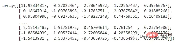
What do the above features represent? Principal component analysis (PCA) projects the data into a low-dimensional space, trying to retain as many differences in the data as possible. While this may help with specific operations, it may also make the data more difficult to understand. , PCA can identify new axes in the data that are linear fusions of the initial features.

Singular Value Decomposition (SVD)

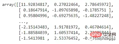
SVD is a linear dimensionality reduction technique that projects features with small data variance into a low-dimensional space. We need to set the number of components to retain after dimensionality reduction. Here we will reduce the dimensionality by 2/3.

from sklearn.decomposition import TruncatedSVD svd = TruncatedSVD(n_compnotallow=int(X_train.shape[1]*0.33)) X_train_svd = svd.fit_transform(X_train) X_test_svd = svd.transform(X_test) X_train_svd

Training the regression model

Now, we will start training and testing the model using the above three types of data (original dataset, PCA and SVD) , and we use multiple models for comparison.

import numpy as np from sklearn.linear_model import LinearRegression from sklearn.neighbors import KNeighborsRegressor from sklearn.svm import SVR from sklearn.tree import DecisionTreeRegressor from sklearn.ensemble import RandomForestRegressor, GradientBoostingRegressor from sklearn.metrics import r2_score, mean_squared_error import time

train_test_ML: This function will complete the repetitive tasks related to the training and testing of the model. The performance of all models was evaluated by calculating rmse and r2_score. and returns a dataset with all details and calculated values. It will also log the time each model took to train and test on its respective dataset.

def train_test_ML(dataset, dataform, X_train, y_train, X_test, y_test): temp_df = pd.DataFrame(columns=['Data Set', 'Data Form', 'Dimensions', 'Model', 'R2 Score', 'RMSE', 'Time Taken']) for i in [LinearRegression, KNeighborsRegressor, SVR, DecisionTreeRegressor, RandomForestRegressor, GradientBoostingRegressor]: start_time = time.time() reg = i().fit(X_train, y_train) y_pred = reg.predict(X_test) r2 = np.round(r2_score(y_test, y_pred), 2) rmse = np.round(np.sqrt(mean_squared_error(y_test, y_pred)), 2) end_time = time.time() time_taken = np.round((end_time - start_time), 2) temp_df.loc[len(temp_df)] = [dataset, dataform, X_train.shape[1], str(i).split('.')[-1][:-2], r2, rmse, time_taken] return temp_df

Original data:

original_df = train_test_ML('AirQualityUCI', 'Original', X_train, y_train, X_test, y_test) original_df

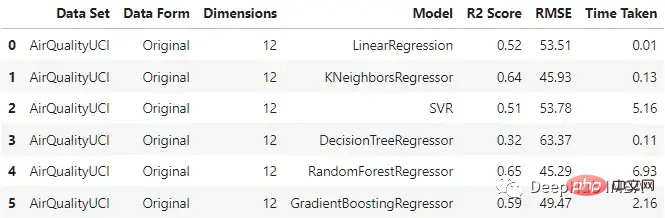
It can be seen that KNN regressor and random forest perform relatively well when inputting original data, and the training time of random forest is the longest.

PCA

pca_df = train_test_ML('AirQualityUCI', 'PCA Reduced', X_train_pca, y_train, X_test_pca, y_test) pca_df

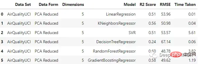
与原始数据集相比，不同模型的性能有不同程度的下降。梯度增强回归和支持向量回归在两种情况下保持了一致性。这里一个主要的差异也是预期的是模型训练所花费的时间。与其他模型不同的是，SVR在这两种情况下花费的时间差不多。

SVD

svd_df = train_test_ML('AirQualityUCI', 'SVD Reduced', X_train_svd, y_train, X_test_svd, y_test) svd_df

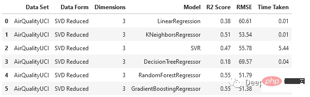
与PCA相比，SVD以更大的比例降低了维度，随机森林和梯度增强回归器的表现相对优于其他模型。

回归模型分析

对于这个数据集，使用主成分分析时，数据维数从12维降至5维，使用奇异值分析时，数据降至3维。

• 就机器学习性能而言，数据集的原始形式相对更好。造成这种情况的一个潜在原因可能是，当我们使用这种技术降低维数时，在这个过程中会发生信息损失。
• 但是线性回归、支持向量回归和梯度增强回归在原始和PCA案例中的表现是一致的。
• 在我们通过SVD得到的数据上，所有模型的性能都下降了。
• 在降维情况下，由于特征变量的维数较低，模型所花费的时间减少了。

将类似的过程应用于其他六个数据集进行测试，得到以下结果:

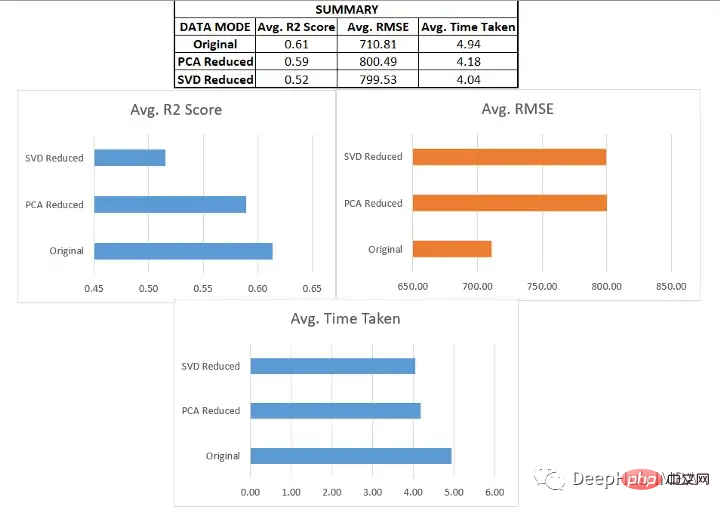
我们在各种数据集上使用了SVD和PCA，并对比了在原始高维特征空间上训练的回归模型与在约简特征空间上训练的模型的有效性

• 原始数据集始终优于由降维方法创建的低维数据。这说明在降维过程中可能丢失了一些信息。
• 当用于更大的数据集时，降维方法有助于显著减少数据集中的特征数量，从而提高机器学习模型的有效性。对于较小的数据集，改影响并不显著。
• 模型的性能在original和pca_reduced两种模式下保持一致。如果一个模型在原始数据集上表现得更好，那么它在PCA模式下也会表现得更好。同样，较差的模型也没有得到改进。
• 在SVD的情况下，模型的性能下降比较明显。这可能是n_components数量选择的问题，因为太小数量肯定会丢失数据。
• 决策树在SVD数据集时一直是非常差的，因为它本来就是一个弱学习器

训练分类模型

对于分类我们将使用另一种降维方法：LDA。机器学习和模式识别任务经常使用被称为线性判别分析(LDA)的降维方法。这种监督学习技术旨在最大化几个类或类别之间的距离，同时将数据投影到低维空间。由于它的作用是最大化类之间的差异，因此只能用于分类任务。

from sklearn.linear_model import LogisticRegression from sklearn.neighbors import KNeighborsClassifier from sklearn.svm import SVC from sklearn.tree import DecisionTreeClassifier from sklearn.ensemble import RandomForestClassifier, GradientBoostingClassifier from sklearn.metrics import accuracy_score, f1_score, recall_score, precision_score

继续我们的训练方法

def train_test_ML2(dataset, dataform, X_train, y_train, X_test, y_test): temp_df = pd.DataFrame(columns=['Data Set', 'Data Form', 'Dimensions', 'Model', 'Accuracy', 'F1 Score', 'Recall', 'Precision', 'Time Taken']) for i in [LogisticRegression, KNeighborsClassifier, SVC, DecisionTreeClassifier, RandomForestClassifier, GradientBoostingClassifier]: start_time = time.time() reg = i().fit(X_train, y_train) y_pred = reg.predict(X_test) accuracy = np.round(accuracy_score(y_test, y_pred), 2) f1 = np.round(f1_score(y_test, y_pred, average='weighted'), 2) recall = np.round(recall_score(y_test, y_pred, average='weighted'), 2) precision = np.round(precision_score(y_test, y_pred, average='weighted'), 2) end_time = time.time() time_taken = np.round((end_time - start_time), 2) temp_df.loc[len(temp_df)] = [dataset, dataform, X_train.shape[1], str(i).split('.')[-1][:-2], accuracy, f1, recall, precision, time_taken] return temp_df

开始训练

from sklearn.discriminant_analysis import LinearDiscriminantAnalysis lda = LinearDiscriminantAnalysis() X_train_lda = lda.fit_transform(X_train, y_train) X_test_lda = lda.transform(X_test)

预处理、分割和数据集的缩放，都与回归部分相同。在对8个不同的数据集进行新联后我们得到了下面结果:

分类模型分析

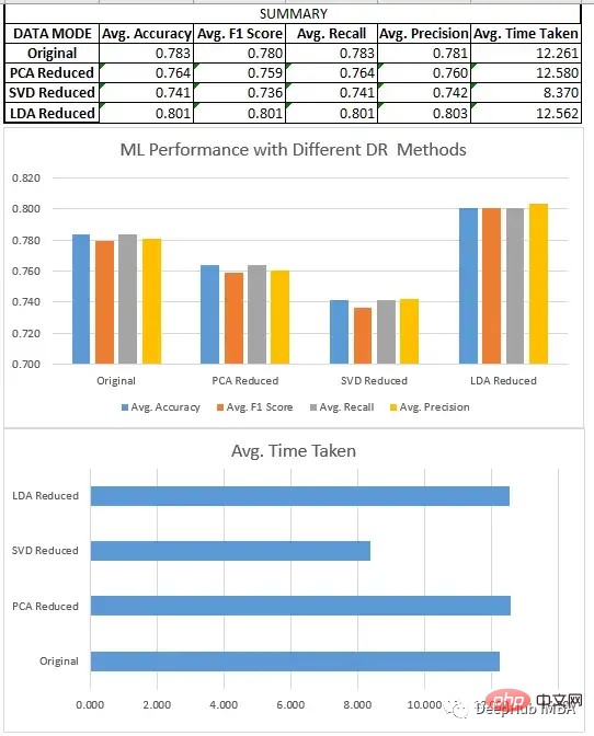
我们比较了上面所有的三种方法SVD、LDA和PCA。

• LDA数据集通常优于原始形式的数据和由其他降维方法创建的低维数据，因为它旨在识别最有效区分类的特征的线性组合，而原始数据和其他无监督降维技术不关心数据集的标签。
• 降维技术在应用于更大的数据集时，可以极大地减少了数据集中的特征数量，这提高了机器学习模型的效率。在较小的数据集上，影响不是特别明显。除了LDA（它在这些情况下也很有效），因为它们在一些情况下，如二元分类，可以将数据集的维度减少到只有一个。
• 当我们在寻找一定的性能时，LDA可以是分类问题的一个非常好的起点。
• SVD与回归一样，模型的性能下降很明显。需要调整n_components的选择。

总结

我们比较了一些降维技术的性能，如奇异值分解(SVD)、主成分分析(PCA)和线性判别分析(LDA)。我们的研究结果表明，方法的选择取决于特定的数据集和手头的任务。

For regression tasks, we find that PCA generally performs better than SVD. In the case of classification, LDA outperforms SVD and PCA, as well as the original dataset. It is important that Linear Discriminant Analysis (LDA) consistently beats Principal Component Analysis (PCA) in classification tasks, but this does not mean that LDA is a better technique in general. This is because LDA is a supervised learning algorithm that relies on labeled data to locate the most discriminative features in the data, while PCA is an unsupervised technique that does not require labeled data and seeks to maintain as much variance as possible. Therefore, PCA may be better suited for unsupervised tasks or situations where interpretability is critical, while LDA may be better suited for tasks involving labeled data.

While dimensionality reduction techniques can help reduce the number of features in a dataset and improve the efficiency of machine learning models, it is important to consider the potential impact on model performance and result interpretability.

The complete code of this article:

https://github.com/salmankhi/DimensionalityReduction/blob/main/Notebook_25373.ipynb

The above is the detailed content of Comparison of common dimensionality reduction technologies: feasibility analysis of reducing data dimensions while maintaining information integrity. For more information, please follow other related articles on the PHP Chinese website!