


Mixed precision has become a necessity for training large deep learning models, but it also brings many challenges. Converting model parameters and gradients to lower precision data types (such as FP16) can speed up training, but also introduces numerical stability issues. The gradient used for FP16 training is more likely to overflow or be insufficient, resulting in inaccurate calculations by the optimizer and problems such as the accumulator exceeding the data type range.

#In this article, we will discuss the numerical stability issue of mixed precision training. Large training jobs are often put on hold for days to deal with numerical instabilities, causing project delays. So we can introduce Tensor Collection Hook to monitor the gradient conditions during training, so that we can better understand the internal state of the model and identify numerical instability faster.
It is a very good way to understand the internal state of the model in the early training stage to determine whether the model is prone to instability in later training. If gradient instability can be identified in the first few hours of training, , can help us improve a lot of efficiency. So this article provides a series of caveats worth paying attention to, as well as remedies for numerical instabilities.
As deep learning continues to evolve toward larger base models. Large language models like GPT and T5 now dominate NLP, and contrasting models such as CLIP generalize better than traditional supervised models in CV. In particular, CLIP's ability to learn text embeddings means that it can perform zero-shot and few-shot inference beyond the capabilities of past CV models, which have been a challenge to train.
These large models typically involve deep networks of transformers, both visual and textual, and contain billions of parameters. GPT3 has 175 billion parameters, and CLIP is trained on hundreds of terabytes of images. The size of the model and data means that models require weeks or even months to train on large GPU clusters. To speed up training and reduce the number of GPUs required, models are often trained in mixed precision.
Hybrid Precision Training puts some training operations in FP16 instead of FP32. Operations performed in FP16 require less memory and can be processed up to 8 times faster than FP32 on modern GPUs. Although most models trained in FP16 have lower accuracy, they do not show any performance degradation due to over-parameterization.
With the introduction of Tensor Cores by NVIDIA in the Volta architecture, low-precision floating point accelerated training is faster. Because deep learning models have many parameters, the exact value of any one parameter is usually not important. By representing numbers with 16 bits instead of 32 bits, more parameters can be fit in Tensor Core registers at once, increasing parallelism for each operation.

But training for FP16 is challenging. Because FP16 cannot represent numbers whose absolute value is greater than 65,504 or less than 5.96e-8. Deep learning frameworks such as PyTorch come with built-in tools to handle the limitations of FP16 (gradient scaling and automatic mixed precision). But even with these safety checks in place, it's not uncommon for large training jobs to fail because parameters or gradients fall outside the available range. Some components of deep learning play well in FP32, but BN, for example, often requires very fine-grained tuning that can lead to numerical instability within the limits of FP16, or not yield enough accuracy for the model to converge correctly. This means that models cannot be converted blindly to FP16.
So the deep learning framework uses Automatic Mixed Precision (AMP), which trains through a predefined list of FP16 safe operations. AMP only converts parts of the model that are considered safe, while keeping operations that require higher precision in FP32. In addition, in the mixed precision training model, a larger gradient is obtained by multiplying some losses close to zero gradient (below the minimum range of FP16) by a certain value, and then when the optimizer is applied to update the model weights, it will be proportionally downward. Adjustment to solve the problem of too small gradients is called gradient scaling.
The following is an example of a typical AMP training loop in PyTorch.

#Gradient scaler The scaler multiplies the loss by a variable amount. If nan is observed in the gradient, the multiplier is reduced by half until the nan disappears, and then gradually increases the multiplier every 2000 steps by default if no nan occurs. This will keep the gradient within the FP16 range while also preventing the gradient from going to zero.
Despite the best efforts of the frameworks, the tools built into PyTorch and TensorFlow cannot prevent the numerical instability that occurs in FP16.
In the T5 implementation of HuggingFace, model variants produce INF values even after training. In very deep T5 models, attention values accumulate across layers and eventually reach outside the FP16 range, which results in infinite values, such as nan in BN layers. They solved this problem by changing the INF value to the maximum value at FP16 and found that this had a negligible impact on inference.
Another common problem is the limitations of the ADAM optimizer. As a small update, ADAM uses a moving average of the first and second moments of the gradient to adapt the learning rate of each parameter in the model.
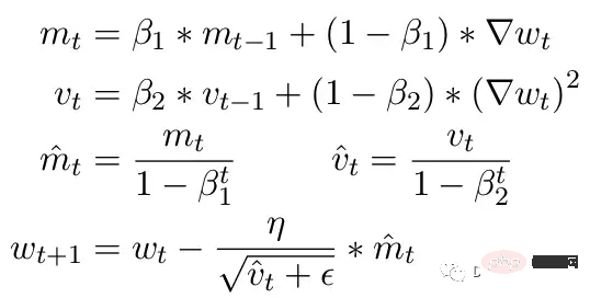
Here Beta1 and Beta2 are the moving average parameters at each moment, usually set to .9 and .999 respectively. Dividing the beta parameter by the power of the number of steps removes the initial bias in the updates. During the update step, a small epsilon is added to the second moment parameter to avoid division by zero errors. The typical default value for epsilon is 1e-8. But the minimum for FP16 is 5.96e-8. This means that if the second moment is too small, the update will be divided by zero. So in PyTorch so that training does not diverge, updates will skip changes in this step. But the problem still exists. Especially in the case of Beta2=.999, any gradient smaller than 5.96e-8 may stop the parameter weight update for a long time, and the optimizer will enter an unstable state.
The advantage of ADAM is that by using these two moments, the learning rate of each parameter can be adjusted. For slower learning parameters, the learning speed can be accelerated, and for fast learning parameters, the learning speed can be slowed down. But if the gradient is calculated to be zero for multiple steps, even a small positive value will cause the model to diverge before the learning rate has time to adjust downwards.
Also PyTorch currently has an issue that automatically changes epsilon to 1e-7 when using mixed precision, which can help prevent the gradient from diverging when moving back to positive values. But doing so brings a new problem. When we know that the gradient is in the same range, increasing ε reduces the optimizer's ability to adapt to the learning rate. Therefore, blindly increasing epsilon cannot solve the problem of training stagnation due to zero gradient.
To further demonstrate the instability that may occur during training, we constructed a series of experiments on the CLIP image model. CLIP is a contrastive learning-based model that simultaneously learns images through a visual transformer and text embeddings describing these images. The comparison component attempts to match the images back to the original description in each batch of data. Since the loss is computed in batches, training on larger batches has been shown to provide better results.
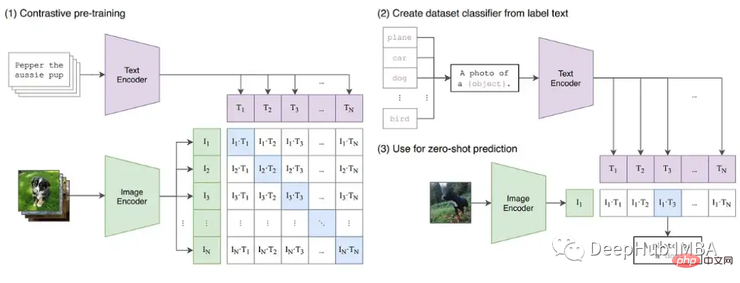
CLIP simultaneously trains two transformers models, a GPT-like language model and a ViT image model. The depth of both models creates opportunities for gradient growth to exceed the FP16 limit. The OpenClip (arxiv 2212.07143) implementation describes training instability when using FP16.
To better understand the internal model state during training, we developed a Tensor Collection Hook (TCH). TCH can wrap a model and periodically collect summary information about weights, gradients, losses, inputs, outputs, and optimizer status.
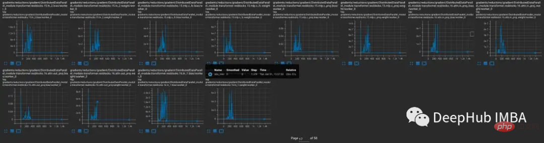
For example, in this experiment, we want to find and record the gradient conditions during training. For example, you might want to collect the gradient norm, minimum, maximum, absolute value, mean, and standard deviation from each layer every 10 steps and visualize the results in TensorBoard.

You can then start TensorBoard with out_dir as the --logdir input.

To reproduce the training instability in CLIP, the Laion 5 billion image dataset used for OpenCLIP training a subset. We wrap the model with TCH and regularly save the model gradients, weights, and optimizer moment states, so that we can observe what happens inside the model when instability occurs.
Starting with the vvi-h-14 variant, the OpenCLIP authors describe a stability issue during training. Starting from the pre-training checkpoint, increase the learning rate to 1-e4, similar to the learning rate in the second half of CLIP training. When training reaches 300 steps, 10 more difficult training batches are intentionally introduced in succession.
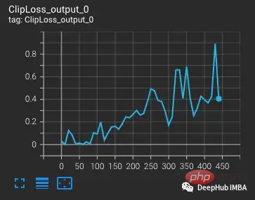
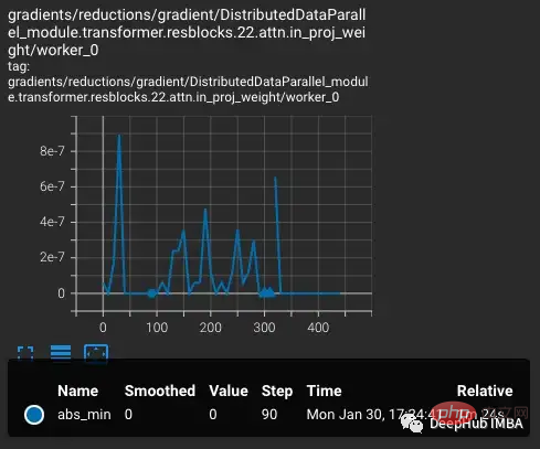
The loss will increase as the learning rate increases, which is expected. When a more difficult situation is introduced at step 300, there is a small, but not large, increase in the loss. The model finds difficult cases but does not update most of the weights in these steps because nan appears in the gradient (shown as a triangle in the second plot). After passing this difficult set of cases, the gradient drops to zero.
What is happening here? Why is the gradient zero? The problem lies in PyTorch’s gradient scaling. Gradient scaling is an important tool in mixed precision training. Because in models with millions or billions of parameters, the gradient of any one parameter is small and often below the minimum range of FP16.
When hybrid precision training was first proposed, deep learning scientists found that their models often trained as expected early in training, but eventually diverge. As training progresses the gradient tends to become smaller and some underflow FP16 goes to zero, making the training unstable.

To solve gradient underflow, early techniques simply multiplied the loss by a fixed amount, calculated the larger gradient, and then Weight updates are adjusted to the same fixed amount (during mixed-precision training, the weights are still stored in FP32). But sometimes this fixed amount is still not enough. And newer techniques, like PyTorch's gradient scaling, start with a larger multiplier, usually 65536. But since this can be so high that large gradients will overflow the FP16 value, the gradient scaler monitors nan gradients that will overflow. If nan is observed, skip the weight update at this step to halve the multiplier and proceed to the next step. This continues until no nan is observed in the gradient. If the gradient scaler does not detect a nan in step 2000, it will try to double the multiplier.
In the example above, the gradient scaler works exactly as expected. We pass it a set of cases where the loss is larger than expected, which creates larger gradients leading to overflow. But the problem is that the multiplier is now low, the smaller gradients are falling to zero, and the gradient scaler does not monitor zero gradients only nan.
The above example may initially seem somewhat intentional, as we intentionally group difficult examples. But after several days of training, in the case of large batches, the probability of generating nan anomalies will definitely increase. So the chance of encountering enough nan to push the gradient to zero is very high. In fact, even if difficult samples are not introduced, it is often found that the gradient is always zero after thousands of training steps.
To further explore when the problem occurs and when it does not, CLIP was compared with CLIP, which is typically trained under mixed precision. The smaller CV model YOLOV5 is compared. The frequency of zero gradients in each layer was tracked during training in both cases.

During the first 9000 steps of training, 5-20% of the layers in CLIP show gradient underflow, while layers in Yolo only show occasional underflow. The underflow rate in CLIP also increases over time, making training less stable.
Using gradient scaling does not solve this problem because the gradient amplitude in the CLIP range is much larger than the gradient amplitude in the YOLO range. In the case of CLIP, while the gradient scaler moves the larger gradients closer to the maximum in FP16, the smallest gradients remain below the minimum.
In some cases, adjusting the parameters of the gradient scaler can help prevent underflow. In the case of CLIP, one could try modifications to start with a larger multiplier and shorten the increase interval.

But we find that the multiplier drops immediately to prevent overflow and force the small gradient back to zero.

One solution to improve the scaling is to make it more adaptable to the parameter range. For example, the paper Adaptive Loss Scaling for Mixed Precision Training recommends performing loss scaling by layer instead of the entire model, which can prevent underflow. Our experiments demonstrate the need for a more adaptive approach. Since the gradients within the CLIP layer still cover the entire FP16 range, scaling needs to be adapted to each individual parameter to ensure training stability. But such detailed scaling requires a lot of memory which reduces the training batch size.
Newer hardware offers more efficient solutions. For example, BFloat16 (BF16) is another 16-bit data type that trades precision for greater range. FP16 handles 5.96e-8 to 65,504, while BF16 can handle 1.17e-38 to 3.39e38, the same range as FP32. However, the accuracy of BF16 is lower than FP16, which will cause some models to not converge. But for large transformers models, BF16 has not been shown to reduce convergence.
We run the same test inserting a batch of difficult observations. In BF16 the gradients spike when hard cases are introduced and then return to regular training because the gradient scaling changes from NaN is not observed in the gradient.

Comparing the CLIP of FP16 and BF16, we found that there are only occasional gradient underflows in BF16.

In PyTorch 1.12 and later, it is possible to enable BF16 with a small change to AMP.

If you need higher precision, you can try the Tensorfloat32 (TF32) data type. TF32, introduced by Nvidia in Ampere GPUs, is a 19-bit floating point that adds the extra range bits of BF16 while retaining the precision of FP16. Unlike FP16 and BF16, it is designed to directly replace FP32, rather than being enabled in mixed precision. To enable TF32 in PyTorch, add two lines at the beginning of training.

It should be noted here: Before PyTorch 1.11, TF32 was enabled by default on GPUs that supported this data type. Starting with PyTorch 1.11, it must be enabled manually. The training speed of TF32 is slower than BF16 and FP16. The theoretical FLOPS is only half of FP16, but it is still much faster than the training speed of FP32.
If you use Amazon AWS: BF16 and TF32 are available on P4d, P4de, G5, Trn1 and DL1 instances.
The example above illustrates how to identify and fix FP16-wide limitations. But these problems often appear later in training. Early in training, when the model generates higher losses and is less sensitive to outliers, as happens in OpenCLIP training, it can take days before problems arise, wasting expensive computational time.
Both FP16 and BF16 have advantages and disadvantages. The limitations of FP16 can lead to unstable and stalled training. However, BF16 provides lower accuracy and may have poorer convergence. So we definitely want to identify models that are susceptible to FP16 instability early in training so we can make informed decisions before instability occurs. So again comparing those models that do and do not exhibit subsequent training instability, two trends can be found.

The YOLO model trained in FP16 and the CLIP model trained in BF16 both show that the gradient underflow rate is generally less than 1%, and the gradient underflow rate is generally less than 1%. It is stable over time.

The CLIP model trained in FP16 has an underflow rate of 5-10% in the first 1000 steps of training and over time Upward trend.
So by using TCH to track the gradient underflow rate, we can identify the trend of higher gradient instability within the first 4-6 hours of training. Switch to BF16 when this trend is observed.
Hybrid precision training is an important part of training existing large-scale base models, but requires special attention to numerical stability. Understanding a model's internal state is important for diagnosing when a model encounters the limitations of mixed-precision data types. By wrapping the model with a TCH, it is possible to track whether parameters or gradients are approaching numerical limits and perform training changes before instability occurs, potentially reducing the number of days of unsuccessful training runs.
The above is the detailed content of How to solve the limitations of mixed precision training of large models. For more information, please follow other related articles on the PHP Chinese website!


![[Web front-end] Node.js quick start](https://img.php.cn/upload/course/000/000/067/662b5d34ba7c0227.png)


