


Translator| Zhao Qingyu
Reviewer| Sun Shujuan
In machine learning, classification has two stages , are the learning stage and the prediction stage respectively. In the learning phase, a model is built based on the given training data; in the prediction phase, the model is used to predict the response given the data. Decision trees are one of the easiest classification algorithms to understand and explain.
In machine learning, classification has two stages, namely the learning stage and the prediction stage. In the learning phase, a model is built based on the given training data; in the prediction phase, the model is used to predict the response given the data. Decision trees are one of the easiest classification algorithms to understand and explain.
The decision tree algorithm is one of the supervised learning algorithms. Unlike other supervised learning algorithms, the decision tree algorithm can be used to solve both regression and classification problems.
The purpose of using a decision tree is to create a training model that predicts the class or value of a target variable by learning simple decision rules inferred from previous data (training data).
In a decision tree, we start from the root of the tree to predict the class label of a record. We compare the value of the root attribute with the recorded attribute, and based on the comparison, we follow the branch corresponding to this value and jump to the next node.
Based on the types of target variables we have, we can divide trees into two types:
1. Categorical variable decision tree: Yes A decision tree of a categorical target variable is called a categorical variable decision tree.
2. Continuous variable decision tree: The target variable of the decision tree is continuous, so it is called a continuous variable decision tree.
Example: Suppose we have a problem of predicting whether a customer will pay a renewal premium to an insurance company. A customer's income is an important variable here, but insurance companies don't have income details for all customers. Now that we know this is an important variable, we can then build a decision tree to predict a customer's revenue based on occupation, product, and various other variables. In this case, we predict that the target variable is continuous.
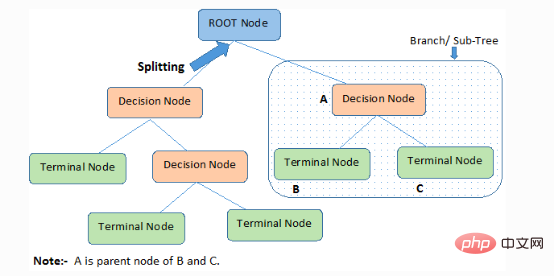
1. Root node (root node): It represents the entire member or sample, which will be further divided into two or more of the same type collection.
2. Splitting): The process of splitting a node into two or more child nodes.
3. Decision Node: When a child node splits into more child nodes, it is called a decision node.
4. Leaf/Terminal Node: A node that cannot be split is called a leaf or terminal node.
5. Pruning: The process in which we delete the child nodes of a decision node is called pruning. Construction can also be seen as the reverse process of separation.
6. Branch/Sub-Tree: A subpart of the entire tree is called a branch or subtree.
7. Parent and Child Node: A node that can be split into child nodes is called a parent node, and a child node is a child node of the parent node.
The decision tree classifies samples in descending order from the root to the leaf/terminal nodes, which provide the classification method of the sample. Each node in the tree acts as a test case for a certain attribute, and each descending direction from the node corresponds to a possible answer to the test case. This process is recursive in nature and is treated the same for each subtree rooted at a new node.
The following are some assumptions we make when using decision trees:
●First, take the entire training set as the root.
●It is best that the feature values can be classified. If these values are continuous, they can be discretized before building the model.
●Records are recursively distributed based on attribute values.
●By using some statistical methods, the corresponding attributes are placed at the root node of the tree or the internal nodes of the tree in order.
The decision tree follows the sum of products expression form. Sum of Products (SOP) is also known as disjunctive normal form. For a class, each branch from the root of the tree to a leaf node with the same class is a conjunction of values, and the different branches ending in the class constitute a disjunction.
The main challenge in the implementation process of decision tree is to determine the attributes of the root node and each level node. This problem is the attribute selection problem. There are currently different attribute selection methods to select the attributes of nodes at each level.
The separation characteristics of decision-making seriously affect the accuracy of the tree. The decision-making criteria of classification trees and regression trees are different.
Decision trees use a variety of algorithms to decide to split a node into two or more child nodes. The creation of child nodes increases the homogeneity of the child nodes. In other words, the purity of the node is increased relative to the target variable. The decision tree separates nodes on all available variables and then selects nodes that can produce many isomorphic child nodes for splitting.
The algorithm is selected based on the type of target variable. Next, let’s take a look at some algorithms used in decision trees:
ID3→(Extension of D3)
C4.5→(Successor of ID3)
CART→(Classification and Regression Tree)
CHAID→(Chi-square automatic interaction detection performs multi-level separation when calculating the classification tree)
MARS →(Multiple adaptive regression splines)
ID3 algorithm uses a top-down greedy search method to build a decision tree through the possible branch space without backtracking. Greedy algorithms, as the name suggests, always make what seems to be the best choice at a certain moment.
1. It uses the original set S as the root node.
2. During each iteration of the algorithm, iterate over the unused attributes in the set S and calculate the entropy (H) and information gain (IG) of the attribute.
3. Then select the attribute with the smallest entropy or the largest information gain.
4. Then separate the set S using the selected attributes to generate subsets of the data.
5. The algorithm continues to iterate over each subset, considering only attributes that have never been selected before on each iteration.
If the data set contains N attributes, then deciding which attribute to place at the root node or at different levels of the tree as an internal node is a complex step. The problem cannot be solved by randomly selecting any node as the root node. If we adopt a random approach, we may get worse results.
To solve this attribute selection problem, researchers have designed some solutions. They suggested using the following criteria:
Calculate the value of each attribute using these criteria, then sort the values and place the attributes in the tree in order, that is, the attributes with high values placed at the root position.
When using information gain as the criterion, we assume that the attributes are categorical, while for the Gini index, we assume that the attributes are continuous.
Entropy is a measure of the randomness of the information being processed. The higher the entropy value, the harder it is to draw any conclusions from the information. Tossing a coin is an example of behavior that provides random information.
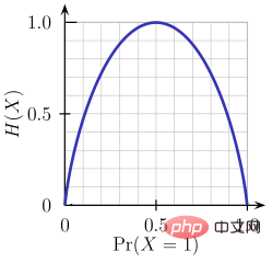
As can be seen from the above figure, when the probability is 0 or 1, the entropy H(X) is zero. Entropy is greatest when the probability is 0.5 because it projects complete randomness in the data.
The rule followed by ID3 is: a branch with an entropy of 0 is a leaf node, and a branch with an entropy greater than 0 needs to be further separated.
The mathematical entropy of a single attribute is expressed as follows:
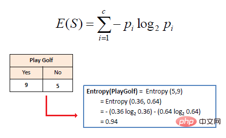
#where S represents the current state, Pi represents the probability of event i in state S or i in state S node Class percentage.
The mathematical entropy of multiple attributes is expressed as follows:
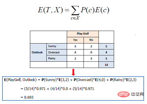
where T represents the current state and X represents the selected attribute
Information gain (IG) is a statistical attribute used to measure the effectiveness of separate training for a given attribute based on the target class. Building a decision tree is the process of finding an attribute that returns the highest information gain and the lowest entropy.
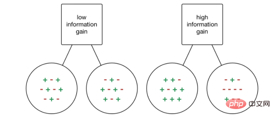
#The increase in information is the decrease in entropy. It calculates the entropy difference before separation and the average entropy difference after separation of the data set based on the given attribute value. The ID3 decision tree algorithm uses the information gain method.
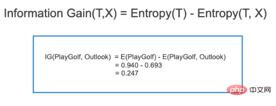
IG is expressed mathematically as follows:
With a simpler approach, we can draw this conclusion:
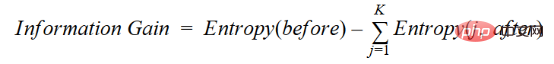
where before is the data set before splitting, K is the number of subsets generated by splitting, and (j, after) is the subset j after splitting.
You can think of the Gini index as a cost function used to evaluate separation in a data set. It is calculated by subtracting the sum of squared probabilities for each class from 1. It favors the case of larger partitions and is easier to implement, while information gain favors the case of smaller partitions with different values.
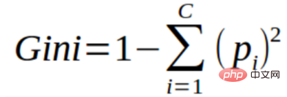
The Gini index is inseparable from the categorical target variable "success" or "failure". It only performs binary separation. The higher the Gini coefficient, the higher the degree of inequality and the stronger the heterogeneity.
The steps to calculate the Gini index separation are as follows:
CART (Classification and Regression Tree) uses the Gini index method to create separation points.
Information gain tends to select attributes with a large number of values as root nodes. This means it prefers properties with a large number of different values.
C4.5 is an improved method of ID3, which uses gain ratio, which is a modification of the information gain to reduce its bias, which is usually the best choice method. Gain rate overcomes the problem of information gain by taking into account the number of branches before doing the splitting. It corrects for information gain by taking into account separate intrinsic information.
Suppose we have a dataset that contains users and their movie genre preferences based on variables such as gender, age group, class, etc. With the help of information gain you will separate in "Gender" (assuming it has the highest information gain), now the variables "Age Group" and "Rating" may be equally important, with the help of gain ratio we can choose Properties that are separated in the next layer.
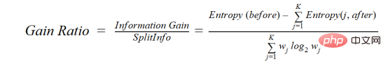
where before is the data set before separation, K is the number of subsets generated by separation, (j, after) is the subset after separation j.
Variance reduction is an algorithm used for continuous target variables (regression problems). The algorithm uses the standard variance formula to choose the best separation. Choose the separation with lower variance as the criterion for separating the population:
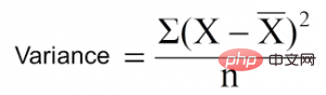
is the mean, X is the actual value, and n is the number of values.
Steps to calculate variance:
CHAID is the abbreviation of Chi-squared Automatic Interaction Detector. This is one of the older tree classification methods. Find the statistically significant difference between a child node and its parent node. We measure it by the sum of squared differences between the observed and expected frequencies of the target variable.
It works with the categorical target variable "Success" or "Failure". It can perform two or more separations. The higher the chi-square value, the more statistically significant the difference between the child node and the parent node. It generates a tree called CHAID.
In mathematics, Chi-squared is expressed as:
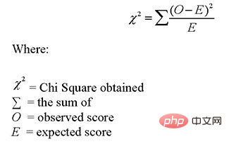
The steps to calculate Chi-squared are as follows:
There is a decision tree Common problem, especially with a tree full of columns. Sometimes it looks like the tree memorized the training data set. If a decision tree had no constraints, it would give you 100% accuracy on the training data set, because in the worst case, it would end up producing one leaf for every observation. Therefore, this affects accuracy when predicting samples that are not part of the training set.
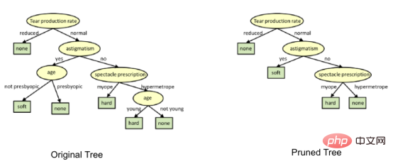
Here I introduce two methods to eliminate overfitting, namely pruning decision trees and random forests.
The separation process will produce a fully grown tree until the stopping criterion is reached. However, mature trees are likely to overfit the data, resulting in poor accuracy on unseen data.

import numpy as np
import matplotlib.pyplot as plt
import pandas as pd
After that, we use the following method to load the data set. It includes 5 attributes, user id, gender, age, estimated salary and purchase status.
data = pd.read_csv('/Users/ML/DecisionTree/Social.csv')
data.head()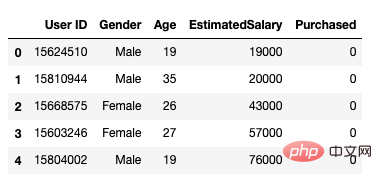
Figure 1 Dataset
We only combine age and prediction Estimated salary is used as our independent variable X because other characteristics such as gender and user ID are irrelevant and have no impact on a person's purchasing power, and y is the dependent variable.
feature_cols = ['Age','EstimatedSalary' ]X = data.iloc[:,[2,3]].values
y = data.iloc[:,4].values
The next step is to separate the data set into training and test sets.
from sklearn.model_selection import train_test_split
X_train, X_test, y_train, y_test =train_test_split(X,y,test_size = 0.25, random_state= 0)
Next perform feature scaling
#feature scaling
from sklearn.preprocessing import StandardScaler
sc_X = StandardScaler()
X_train = sc_X.fit_transform(X_train)
X_test = sc_X.transform(X_test)
Fit the model to the decision tree in the classifier.
from sklearn.tree import DecisionTreeClassifier
classifier = DecisionTreeClassifier()
classifier = classifier.fit(X_train,y_train)
Make predictions and check accuracy.
#prediction
y_pred = classifier.predict(X_test)#Accuracy
from sklearn import metricsprint('Accuracy Score:', metrics.accuracy_score(y_test,y_pred))The decision tree classifier has an accuracy of 91%.
Confusion Matrix
from sklearn.metrics import confusion_matrix
cm = confusion_matrix(y_test, y_pred)Output:
array([[64,4],
 [ 2, 30]])
from matplotlib.colors import ListedColormap
X_set, y_set = X_test, y_test
X1, X2 = np.meshgrid(np.arange(start = X_set[:,0].min()-1, stop= X_set[:,0].max()+1, step = 0.01),np.arange(start = X_set[:,1].min()-1, stop= X_set[:,1].max()+1, step = 0.01))
plt.contourf(X1,X2, classifier.predict(np.array([X1.ravel(), X2.ravel()]).T).reshape(X1.shape), alpha=0.75, cmap = ListedColormap(("red","green")))plt.xlim(X1.min(), X1.max())
plt.ylim(X2.min(), X2.max())for i,j in enumerate(np.unique(y_set)):
plt.scatter(X_set[y_set==j,0],X_set[y_set==j,1], c = ListedColormap(("red","green"))(i),label = j)
plt.title("Decision Tree(Test set)")
plt.xlabel("Age")
plt.ylabel("Estimated Salary")
plt.legend()
plt.show()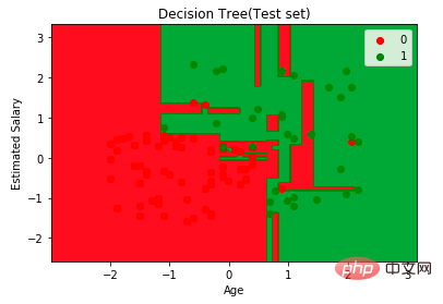 ##Next, imagine this tree
conda install python-graphviz
pip install pydotplus
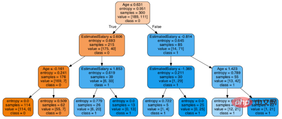
export_graphviz function converts the decision tree classifier to a point file, and pydotplus converts the point file to png or in The form displayed on Jupyter is implemented as follows:
from sklearn.tree import export_graphviz
from sklearn.externals.six import StringIO
from IPython.display import Image
import pydotplusdot_data = StringIO()
export_graphviz(classifier, out_file=dot_data,
filled=True, rounded=True,
special_characters=True,feature_names = feature_cols,class_names=['0','1'])
graph = pydotplus.graph_from_dot_data(dot_data.getvalue())
Image(graph.create_png())
在决策树形图中,每个内部节点都有一个分离数据的决策规则。Gini代表基尼系数,它代表了节点的纯度。当一个节点的所有记录都属于同一个类时,您可以说它是纯节点,这种节点称为叶节点。
在这里,生成的树是未修剪的。这棵未经修剪的树不容易理解。在下一节中,我会通过修剪的方式来优化树。
criteria: 该选项默认配置是Gini,我们可以通过该项选择合适的属性选择方法,该参数允许我们使用different-different属性选择方式。支持的标准包含基尼指数的“基尼”和信息增益的“熵”。
splitter: 该选项默认配置是" best ",我们可以通过该参数选择合适的分离策略。支持的策略包含“best”(最佳分离)和“random”(最佳随机分离)。
max_depth:默认配置是None,我们可以通过该参数设置树的最大深度。若设置为None,则节点将展开,直到所有叶子包含的样本小于min_samples_split。最大深度值越高,过拟合越严重,反之,过拟合将不严重。
在Scikit-learn中,只有通过预剪枝来优化决策树分类器。树的最大深度可以用作预剪枝的控制变量。
# Create Decision Tree classifer object
classifier = DecisionTreeClassifier(criterion="entropy", max_depth=3)# Train Decision Tree Classifer
classifier = classifier.fit(X_train,y_train)#Predict the response for test dataset
y_pred = classifier.predict(X_test)# Model Accuracy, how often is the classifier correct?
print("Accuracy:",metrics.accuracy_score(y_test, y_pred))至此分类率提高到94%,相对之前的模型来说,其准确率更高。现在让我们再次可视化优化后的修剪后的决策树。
dot_data = StringIO()
export_graphviz(classifier, out_file=dot_data,
filled=True, rounded=True,
special_characters=True, feature_names = feature_cols,class_names=['0','1'])
graph = pydotplus.graph_from_dot_data(dot_data.getvalue())
Image(graph.create_png())
上图是经过修剪后的模型,相对之前的决策树模型图来说,其更简单、更容易解释和理解。
在本文中,我们讨论了很多关于决策树的细节,它的工作方式,属性选择措施,如信息增益,增益比和基尼指数,决策树模型的建立,可视化,并使用Python Scikit-learn包评估和优化决策树性能,这就是这篇文章的全部内容,希望你们能喜欢它。
赵青窕,51CTO社区编辑,从事多年驱动开发。
原文标题:Decision Tree Algorithm, Explained,作者:Nagesh Singh Chauhan
The above is the detailed content of Anatomy of Decision Tree Algorithm. For more information, please follow other related articles on the PHP Chinese website!


![[Web front-end] Node.js quick start](https://img.php.cn/upload/course/000/000/067/662b5d34ba7c0227.png)


