
Autonomous driving is a gradual transition from the prediction stage to the industrialization stage. The specific performance can be divided into four points. First of all, in the context of big data, the scale of data sets is rapidly expanding. As a result, details of prototypes previously developed on small-scale data sets will be largely filtered out, and only work that can be effective on large-scale data will be left. The second is the switching of focus, from monocular to multi-view scenes, which leads to an increase in complexity. Then there is the tendency towards application-friendly designs, such as the transfer of the output space from image space to BEV space.
The last thing is to change from purely pursuing accuracy to gradually considering reasoning speed at the same time. At the same time, rapid response is required in autonomous driving scenarios, so the performance requirements will consider speed. In addition, more consideration is given to how to deploy to edge devices.
Another part of the background is that in the past 10 years, visual perception has developed rapidly driven by deep learning. There has been a lot of work and some work in mainstream directions such as classification, detection, and segmentation. A fairly mature paradigm. In the development process of visual perception in autonomous driving scenarios, aspects such as target definition of feature encoding, perception paradigm and supervision have drawn heavily on these mainstream directions. Therefore, before committing to autonomous driving perception, these mainstream directions should be explored. Dabble a bit.
Against these backgrounds, a large number of 3D target detection work on large-scale data sets has emerged in the past year, as shown in Figure 1 (the ones marked in red are the first ones) algorithm).

Figure 1 Three-dimensional target detection development in the past year
The difference between visual perception in autonomous driving scenarios and mainstream vision mainly lies in the given The target definition space is different. The target of mainstream visual perception is defined in the image space, while the target of the autonomous driving scene is defined in the 3-dimensional space. When the inputs are all images, obtaining the results in the 3-dimensional space requires a Lift process. This is the core issue of visual perception for autonomous driving.
We can divide the method of solving the Lift object problem into input, intermediate features and output. An example of the input level is perspective change. The principle is to use images to reason about depth information, and then Use depth information to project the RGB values of the image into a three-dimensional space to obtain a colored point cloud. The related work of point cloud detection will be followed later.
Currently, the more promising ones are feature-level transformation or feature-level lift. For example, DETR3D, these all perform spatial changes at the feature level. The advantage of feature-level transformation is that it can avoid duplication. To extract image-level features, the calculation amount is small, and it can also avoid the problem of output-level look-around result fusion. Of course, feature-level conversion will also have some typical problems. For example, some strange OPs are usually used, which makes deployment unfriendly.
At present, the Lift process at the feature level is relatively robust mainly based on depth and attention mechanism strategies, the representative ones are BEVDet and DETR3D respectively. The depth-based strategy completes a process of Lift by calculating the depth of each point of the image, and then projecting the features into a 3-dimensional space according to the camera's imaging model. The strategy based on the attention mechanism is to pre-define an object in the 3-dimensional space as a query, find the image features corresponding to the midpoint of the three-dimensional space as key and value through internal and external parameters, and then calculate a 3-dimensional object through attention. A characteristic of an object in space.
All current algorithms are basically highly dependent on the camera model, whether it is based on depth or attention mechanism, which will lead to sensitivity to calibration and generally complicated calculation process. . Algorithms that abandon camera models often lack robustness, so this aspect is not yet fully mature.
Temporal information can effectively improve the effect of target detection. For autonomous driving scenarios, timing has a deeper meaning because the speed of the target is one of the main perception targets in the current scenario. The focus of speed lies in change. Single frame data does not have sufficient change information, so modeling is needed to provide change information in the time dimension. The existing point cloud time series modeling method is to mix the point clouds of multiple frames as input, so that a relatively dense point cloud can be obtained, making the detection more accurate. In addition, multi-frame point clouds contain continuous information. Later, during the network training process, BP is used to learn how to extract this continuous information to solve tasks such as speed estimation that require continuous information.
The timing modeling method of visual perception mainly comes from BEVDet4D and BEVFormer. BEVDet4D provides continuous information for subsequent networks by simply fusing a feature of two frames. The other path is based on attention, providing both single-temporal frame and counterclockwise features as an object of query, and then querying these two features simultaneously through attention to extract timing information.
One of the biggest shortcomings of autonomous driving visual perception compared to radar perception is the accuracy of depth estimation. Spend. The paper "probabilistic and geometric depth: detecting objects in perspective" studies the impact of different factors on performance scores by replacing the GT method. The main conclusion from the analysis is that accurate depth estimation can bring significant performance improvements.
But depth estimation is a major bottleneck in current visual perception. There are currently two main ways to improve it. One is to use geometric constraints in PGD to perform prediction on the depth map. refine. The other is to use lidar as supervision to obtain a more robust depth estimate.
The current solution that is superior in the process, BEVDepth, uses the depth information provided by lidar during the training process to supervise the depth estimation during the change process and the main task of perception At the same time.
#Multi-tasking is the hope in one A unified framework is used to complete a variety of perception tasks. Through this calculation, the purpose of saving resources or accelerating computational reasoning can be achieved. However, the current methods basically achieve multi-tasking simply by processing the features at different levels after obtaining a unified feature. There is a common problem of performance degradation after task merging. Multimodality is also almost universal in finding a form that can be directly fused in the entire judgment, and then achieving a simple fusion
BEVDet network is shown in Figure 2. The feature extraction process mainly converts a feature of the extracted image space into a feature of the BEV space, and then further encodes this feature. , obtain a feature that can be used for prediction, and finally use dense prediction to predict the target.

Figure 2 BEVDet network structure
The perspective change module process is divided into two Step by step, first assume that the size of the feature to be transformed is VxCxHxW, and then predict a depth in a classification manner in the image space. For each pixel, a D-dimensional depth distribution is obtained. Then you can use these two to combine different depths. The feature is rendered to obtain a visual feature, then the camera model is used to project it into a 3-dimensional space, the 3-dimensional space is voxelized, and then the splat process is performed to obtain the BEV feature.
A very important feature of the perspective change module is that it plays a mutual isolation role in data slowdown. Specifically, through the internal parameters of the camera, a point on the camera coordinate system can be obtained by projecting it into a 3-dimensional space. When the data augmentation is applied to a point in the image space, in order to maintain the coordinates of the point on the camera coordinate system Invariant, you need to do an inverse transformation, that is, a coordinate on the camera coordinate system is unchanged before and after augmentation, which has a mutual isolation effect. The disadvantage of mutual isolation is that the augmentation of the image space does not regularize the learning of the BEV space. The advantage can improve the robustness of the BEV space learning.
We start from the experiment Several important conclusions can be drawn from the above. First, after using the BEV space encoder, the algorithm is more likely to fall into overfitting. Another conclusion is that the expansion of BEV space will have a greater impact on performance than the expansion of image space.
There is also the correlation between the target size of the BEV space and the category height. At the same time, the small overlap length between the targets will cause some problems. It is observed that the non-polar objects designed in the image space are Large value suppression methods are not optimal. The core of the simultaneous acceleration strategy is to use parallel computing methods to allocate independent threads to different small computing tasks to achieve the purpose of parallel computing acceleration. The advantage is that there is no additional video memory overhead.
BEVDet4D network structure is shown in Figure 3. The main focus of this network is how to apply the features of the reverse-time frame to the current frame. We select the input feature as a retained object, but do not select this image feature, because the target variables are all defined in the BEV space, and the image The characteristics of are not suitable for direct timing modeling. At the same time, the features behind the BEV Encoder are not selected as continuous fusion features, because we need to extract a continuous feature in the BEV Encoder.
Considering that the features output by the perspective change module are relatively sparse, an additional BEV Encoder is connected after the perspective change to extract preliminary BEV features, and then conduct a time series modeling. During timing fusion, we simply splice the features of the counter-clockwise frame with the current needle by aligning them to complete the timing fusion. In fact, we here leave the task of extracting the timing features to the later ones. BEV do it.
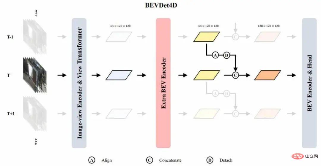
Figure 3 BEVDet4D network structure
How to design and network structure Match the target variable? Before that, we first need to understand some key characteristics of the network. The first is the receptive field of the feature. Because the network learns through BP, the receptive field of the feature is determined by the output space.
The output space of the autonomous driving perception algorithm is generally defined as a space within a certain range around the vehicle. The feature map can be regarded as a uniform distribution on the continuous space, with the corner points Aligned to a discrete sample. Since the receptive field of the feature map is defined within a certain range around the self-car, it will change with the movement of the self-car. Therefore, at two different time nodes, the receptive field of the feature map has a certain value in the world coordinate system. Certain offset.
If the two features are directly spliced together, the position of the static target in the two feature maps is different, and the offset of the dynamic target in the two feature maps It is equal to the offset of the self-test plus the offset of the dynamic target in the world coordinate system. According to a principle of pattern consistency, since the offset of the target in the spliced features is related to the self-vehicle, when setting the learning goal of the network, it should be the change in the position of the target in these two feature maps. .
According to the following formula, it can be deduced that a learning target is not related to the self-test movement, but is only related to a movement of the target in the world coordinate system.

The difference between the learning goals we derived from the above and the learning goals of current mainstream methods is that the time component is removed, and the speed is equal to displacement/time, but these two features do not provide time-related clues. Therefore, if you want to learn this speed target, the network needs to accurately estimate the time component, which increases the difficulty of learning. In practice, we can set the time between two frames as a constant value during the training process. A constant time interval network can be learned by learning BP.
In the augmentation of the time domain, we randomly use different time intervals during the training process. At different time intervals, the offset of the target in the two pictures Different, the target offset of learning is also different, so as to achieve the Lupine effect of the model on different offsets. At the same time, the model has a certain sensitivity to the offset of the target, that is, if the interval is too small, the change between two frames will be difficult to perceive if it is too small. Therefore, choosing an appropriate time interval during testing can effectively improve the generalization performance of the model.
This article uses radar to get a robust Depth estimation, as shown in Figure 4. It uses point clouds to supervise the depth distribution in the change module. This supervision is sparse. This sparseness is dense compared to the depth supervision provided by the target, but it does not reach every pixel. An accurate deep supervision is also relatively sparse. However, more samples can be provided to improve the generalization performance of this depth estimation.
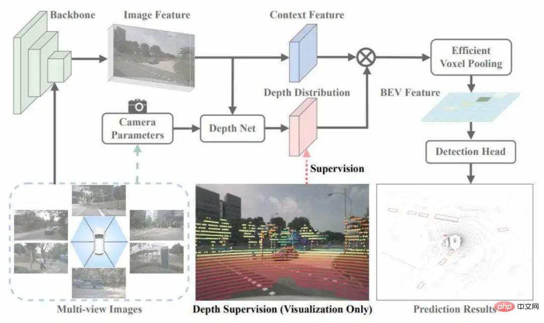
Figure 4 BEVDepth network structure
Another aspect of this work The feature and depth are divided into two branches for estimation, and an additional residual network is added to the depth estimation branch to increase the receptive field of the depth estimation branch. Researchers believe that the accuracy of the internal and external parameters of the camera will cause the context and depth to be misaligned. When the depth estimation network is not powerful enough, there will be a certain loss of accuracy.
Finally, the internal parameters of this camera are used as a depth estimation branch input, and a method similar to NSE is used to adjust the channel of the input feature at the channel level. This can Effectively improve the network's robustness to different camera internal parameters.
First of all, the visual perception of autonomous driving ultimately serves deployment, and during deployment it will involve data issues and model issues. question. The data problem involves a diversity issue and data annotation, because manual annotation is very expensive, so we will see if automated annotation can be achieved in the future.
At present, the labeling of dynamic targets is unprecedented. For static targets, a partial or semi-automatic labeling can be obtained through 3D reconstruction. In terms of models, the current model design is not robust to calibration or is sensitive to calibration. So how to make the model robust to calibration or independent of calibration is also a question worth thinking about.
The other is the issue of network structure acceleration. Can a general OP be used to achieve a change in perspective? This issue will affect the network acceleration process.
The above is the detailed content of A brief analysis of the latest technical routes for visual autonomous driving. For more information, please follow other related articles on the PHP Chinese website!


