Summary of important knowledge points related to machine learning regression models

1. What are the assumptions of linear regression?

Linear regression has four assumptions:

• Linear: There should be a linear relationship between the independent variable (x) and the dependent variable (y), which means that changes in the x value also should change the y value in the same direction.
• Independence: Features should be independent of each other, which means minimal multicollinearity.
• Normality: Residuals should be normally distributed.
• Homoskedasticity: The variance of the data points around the regression line should be the same for all values.

2. What is residual and how is it used to evaluate regression models?

The residual refers to the error between the predicted value and the observed value. It measures the distance of the data points from the regression line. It is calculated by subtracting predicted values from observed values.

Residual plots are a good way to evaluate regression models. It is a graph that shows all the residuals on the vertical axis and the features on the x-axis. If the data points are randomly scattered on lines with no pattern, then a linear regression model fits the data well, otherwise we should use a nonlinear model.

3. How to distinguish between linear regression model and nonlinear regression model?

Both are types of regression problems. The difference between the two is the data they are trained on.

The linear regression model assumes a linear relationship between features and labels, which means if we take all the data points and plot them into a linear (straight) line it should fit the data.

Nonlinear regression models assume that there is no linear relationship between variables. Nonlinear (curvilinear) lines should separate and fit the data correctly.

Three best ways to find out if your data is linear or non-linear -

1. Residual plot
2. Scatter points Figure
3. Assuming the data is linear, a linear model is trained and evaluated by accuracy.

4. What is multicollinearity and how does it affect model performance?

Multicollinearity occurs when certain features are highly correlated with each other. Correlation refers to a measure that indicates how one variable is affected by changes in another variable.

If an increase in feature a leads to an increase in feature b, then the two features are positively correlated. If an increase in a causes a decrease in feature b, then the two features are negatively correlated. Having two highly correlated variables on the training data will lead to multicollinearity as its model cannot find patterns in the data, resulting in poor model performance. Therefore, before training the model, we must first try to eliminate multicollinearity.

5. How do outliers affect the performance of linear regression models?

Outliers are data points whose values differ from the average range of the data points. In other words, these points are different from the data or outside the 3rd criterion.

# Linear regression models attempt to find a best-fit line that reduces residuals. If the data contains outliers, the line of best fit will shift a bit toward the outliers, increasing the error rate and resulting in a model with a very high MSE.

6. What is the difference between MSE and MAE?

MSE stands for mean square error, which is the squared difference between the actual value and the predicted value. And MAE is the absolute difference between the target value and the predicted value.

MSE penalizes big mistakes, MAE does not. As the values of both MSE and MAE decrease, the model tends to a better fitting line.

7. What are L1 and L2 regularization and when should they be used?

In machine learning, our main goal is to create a general model that can perform better on training and test data, but when there is very little data, basic linear regression models tend to overfit. together, so we will use l1 and l2 regularization.

L1 regularization or lasso regression works by adding the absolute value of the slope as a penalty term within the cost function. Helps remove outliers by removing all data points with slope values less than a threshold.

L2 regularization or ridge regression adds a penalty term equal to the square of the coefficient size. It penalizes features with higher slope values.

l1 and l2 are useful when the training data is small, the variance is high, the predicted features are larger than the observed values, and multicollinearity exists in the data.

8. What does heteroskedasticity mean?

It refers to the situation where the variances of the data points around the best-fit line are different within a range. It results in uneven dispersion of residuals. If it is present in the data, then the model tends to predict invalid output. One of the best ways to test for heteroskedasticity is to plot the residuals.

One of the biggest causes of heteroskedasticity within data is the large differences between range features. For example, if we have a column from 1 to 100000, then increasing the values by 10% will not change the lower values, but will make a very large difference at the higher values, thus producing a large variance difference. data point.

9. What is the role of the variance inflation factor?

The variance inflation factor (vif) is used to find out how well an independent variable can be predicted using other independent variables.

Let's take example data with features v1, v2, v3, v4, v5 and v6. Now, to calculate the vif of v1, consider it as a predictor variable and try to predict it using all other predictor variables.

If the value of VIF is small, it is better to remove the variable from the data. Because smaller values indicate high correlation between variables.

10. How does stepwise regression work?

Stepwise regression is a method of creating a regression model by removing or adding predictor variables with the help of hypothesis testing. It predicts the dependent variable by iteratively testing the significance of each independent variable and removing or adding some features after each iteration. It runs n times and tries to find the best combination of parameters that predicts the dependent variable with the smallest error between the observed and predicted values.

It can manage large amounts of data very efficiently and solve high-dimensional problems.

11. In addition to MSE and MAE, are there any other important regression indicators?

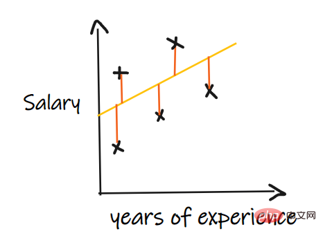
We use a regression problem to introduce these indicators, where our input is work experience and the output is salary. The graph below shows a linear regression line drawn to predict salary.

1. Mean absolute error (MAE):

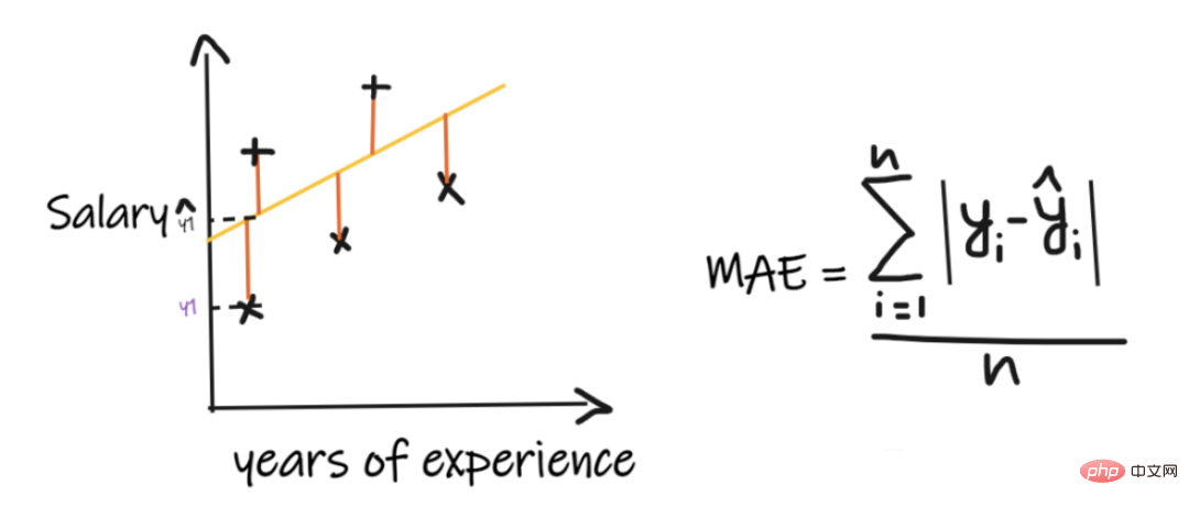
Mean absolute error (MAE) is the simplest regression measure. It adds the difference between each actual and predicted value and divides it by the number of observations. In order for a regression model to be considered a good model, the MAE should be as small as possible.

The advantages of MAE are:

Simple and easy to understand. The result will have the same units as the output. For example: If the unit of the output column is LPA, then if the MAE is 1.2, then we can interpret the result as 1.2LPA or -1.2LPA, MAE is relatively stable to outliers (compared to some other regression indicators, MAE is affected by outliers smaller).

The disadvantage of MAE is:

MAE uses a modular function, but the modular function is not differentiable at all points, so it cannot be used as a loss function in many cases.

2. Mean square error (MSE):

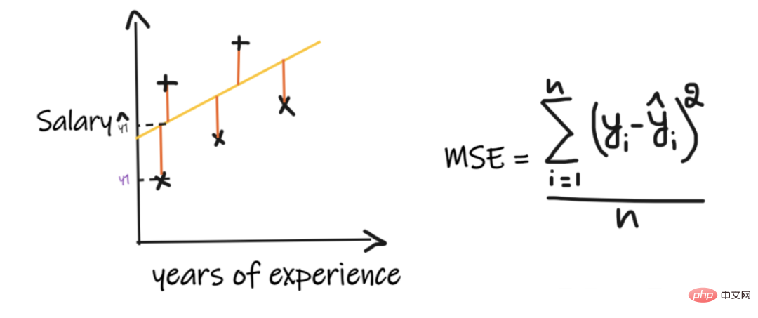
MSE takes the difference between each actual value and the predicted value, then squares the difference and adds them together, finally dividing by the number of observations. In order for a regression model to be considered a good model, the MSE should be as small as possible.

Advantages of MSE:The square function is differentiable at all points, so it can be used as a loss function.

Disadvantages of MSE:Since MSE uses the square function, the unit of the result is the square of the output. It is therefore difficult to interpret the results. Since it uses a square function, if there are outliers in the data, the differences will also be squared, and therefore, MSE is not stable for outliers.

3. Root mean square error (RMSE):

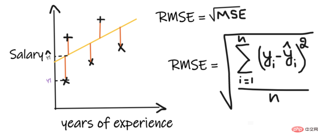
The root mean square error (RMSE) takes the difference between each actual value and the predicted value values, then square the differences and add them, and finally divide by the number of observations. Then take the square root of the result. Therefore, RMSE is the square root of MSE. In order for a regression model to be considered a good model, the RMSE should be as small as possible.

RMSE solves the problem of MSE, the units will be the same as those of the output since it takes the square root, but is still less stable to outliers.

The above indicators depend on the context of the problem we are solving. We cannot judge the quality of the model by just looking at the values of MAE, MSE and RMSE without understanding the actual problem.

4, R2 score:

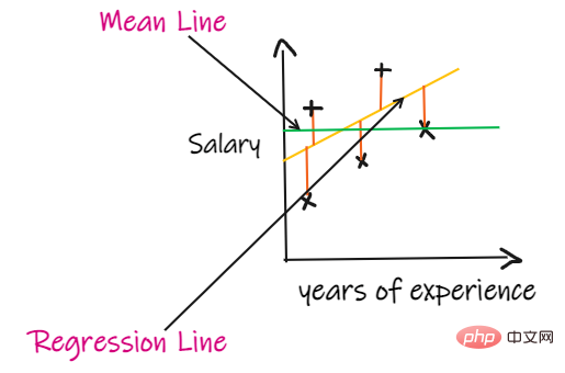
If we don’t have any input data, but want to know how much salary he can get in this company, then we can The best thing to do is give them an average of all employee salaries.

#R2 score gives a value between 0 and 1 and can be interpreted for any context. It can be understood as the quality of the fit.

SSR is the sum of squared errors of the regression line, and SSM is the sum of squared errors of the moving average. We compare the regression line to the mean line.

• #If the R2 score is 0, it means that our model has the same results as the average, so our model needs to be improved.
• If the R2 score is 1, the right-hand side of the equation becomes 0, which can only happen if our model fits each data point without error.
• If the R2 score is negative, it means the right side of the equation is greater than 1, which can happen when SSR > SSM. This means that our model is worst than the average, which means that our model is worse than taking the average to predict

If the R2 score of our model is 0.8, this means that it can be said that the model can Explains 80% of the output variance. That is, 80% of the wage variation can be explained by the input (working years), but the remaining 20% is unknown.

If our model has 2 features, working years and interview scores, then our model can explain 80% of the salary changes using these two input features.

Disadvantages of R2:

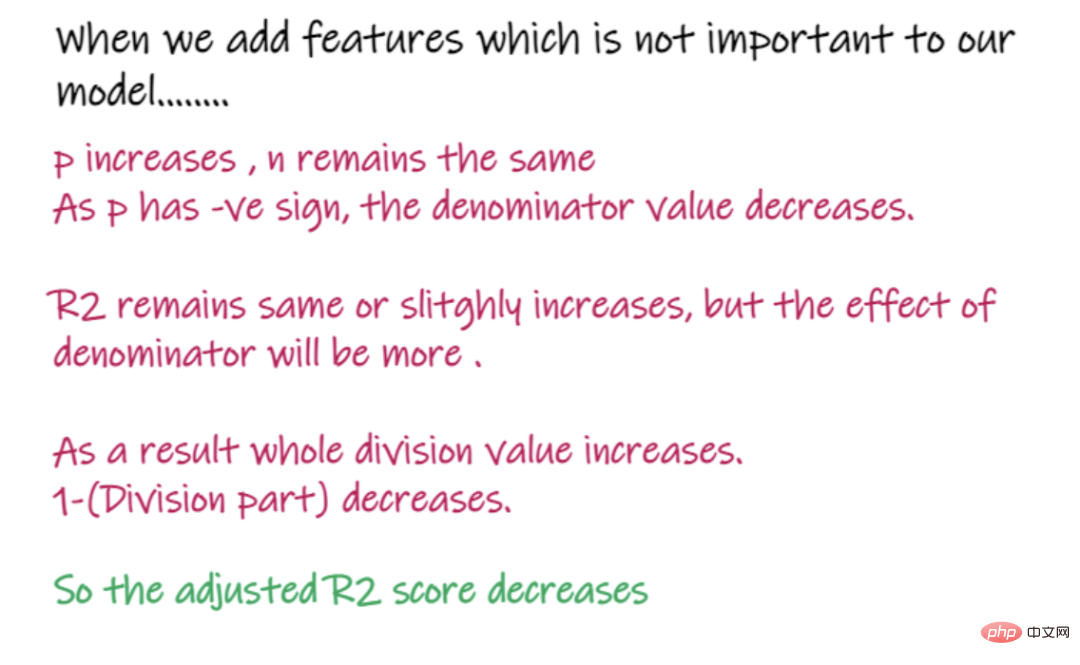
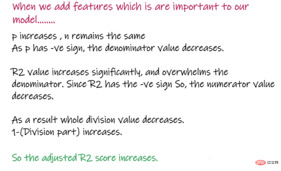
As the number of input features increases, R2 will tend to increase accordingly or remain unchanged, but will never decrease, even if the input features are not useful for our model important (e.g., adding the temperature on the day of the interview to our example, R2 will not decrease even if the temperature is not important to the output).

5. Adjusted R2 score:

In the above formula, R2 is R2, n is the number of observations (rows), and p is the number of independent features. Adjusted R2 solves the problems of R2.

When we add features that are less important to our model, like adding temperature to predict wages.....

When adding features that are important to the model, such as adding interview scores to predict salary...

The above is the regression problem Important knowledge points and the introduction of various important indicators used to solve regression problems and their advantages and disadvantages. I hope it will be helpful to you.

The above is the detailed content of Summary of important knowledge points related to machine learning regression models. For more information, please follow other related articles on the PHP Chinese website!