Summary of nine top-flow regression algorithms and examples-AI-php.cn

Summary of nine top-flow regression algorithms and examples

Linear regression is often the first algorithm people learn for machine learning and data science. It is simple and easy to understand, but due to its limited functionality, it is not the best choice in real business. Most often, linear regression is used as a baseline model to evaluate and compare new methods in research.

When dealing with practical problems, we should know and have tried many other regression algorithms. In this article, learn 9 popular regression algorithms through hands-on exercises using Scikit-learn and XGBoost. The structure of this article is as follows:

Summary of nine top-flow regression algorithms and examples

Written in front

This data uses a well-known data science disclosure hidden in the third-party vega_datasets module of Python data set.

There are quite a lot of data sets in vega_datasets, including statistical data, geographical data, and versions with different data amounts. For example, the flights data set contains multiple versions such as 2k, 5k, 200k, 3m, etc.

The call is to write: df = data('iris') or df = data.iris(). The data exists in the Anaconda3/Lib/site-packages/vega_datasets directory and is stored locally in local_datasets.json There is a description. Local storage includes csv format and json format.

Importing and using data sets

<span style="color: rgb(89, 89, 89); margin: 0px; padding: 0px; background: none 0% 0% / auto repeat scroll padding-box border-box rgba(0, 0, 0, 0);">df</span> <span style="color: rgb(215, 58, 73); margin: 0px; padding: 0px; background: none 0% 0% / auto repeat scroll padding-box border-box rgba(0, 0, 0, 0);">=</span> <span style="color: rgb(89, 89, 89); margin: 0px; padding: 0px; background: none 0% 0% / auto repeat scroll padding-box border-box rgba(0, 0, 0, 0);">data</span>.<span style="color: rgb(0, 92, 197); margin: 0px; padding: 0px; background: none 0% 0% / auto repeat scroll padding-box border-box rgba(0, 0, 0, 0);">cars</span>()<br><span style="color: rgb(89, 89, 89); margin: 0px; padding: 0px; background: none 0% 0% / auto repeat scroll padding-box border-box rgba(0, 0, 0, 0);">df</span>.<span style="color: rgb(0, 92, 197); margin: 0px; padding: 0px; background: none 0% 0% / auto repeat scroll padding-box border-box rgba(0, 0, 0, 0);">head</span>()<br>

Copy after login

Summary of nine top-flow regression algorithms and examples

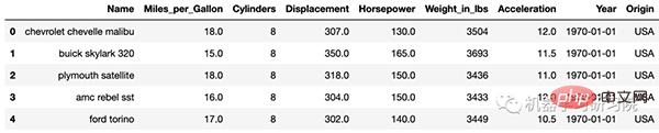
<span style="color: rgb(89, 89, 89); margin: 0px; padding: 0px; background: none 0% 0% / auto repeat scroll padding-box border-box rgba(0, 0, 0, 0);">df</span>.<span style="color: rgb(0, 92, 197); margin: 0px; padding: 0px; background: none 0% 0% / auto repeat scroll padding-box border-box rgba(0, 0, 0, 0);">info</span>()<br>

Copy after login

<span style="color: rgb(215, 58, 73); margin: 0px; padding: 0px; background: none 0% 0% / auto repeat scroll padding-box border-box rgba(0, 0, 0, 0);"><span style="color: rgb(215, 58, 73); margin: 0px; padding: 0px; background: none 0% 0% / auto repeat scroll padding-box border-box rgba(0, 0, 0, 0);">class</span> <span style="color: rgb(102, 153, 0); margin: 0px; padding: 0px; background: none 0% 0% / auto repeat scroll padding-box border-box rgba(0, 0, 0, 0);">'pandas.core.frame.DataFrame'</span><span style="color: rgb(215, 58, 73); margin: 0px; padding: 0px; background: none 0% 0% / auto repeat scroll padding-box border-box rgba(0, 0, 0, 0);">></span><br><span style="color: rgb(89, 89, 89); margin: 0px; padding: 0px; background: none 0% 0% / auto repeat scroll padding-box border-box rgba(0, 0, 0, 0);">RangeIndex</span>: <span style="color: rgb(0, 92, 197); margin: 0px; padding: 0px; background: none 0% 0% / auto repeat scroll padding-box border-box rgba(0, 0, 0, 0);">406</span> <span style="color: rgb(89, 89, 89); margin: 0px; padding: 0px; background: none 0% 0% / auto repeat scroll padding-box border-box rgba(0, 0, 0, 0);">entries</span>, <span style="color: rgb(0, 92, 197); margin: 0px; padding: 0px; background: none 0% 0% / auto repeat scroll padding-box border-box rgba(0, 0, 0, 0);">0</span> <span style="color: rgb(89, 89, 89); margin: 0px; padding: 0px; background: none 0% 0% / auto repeat scroll padding-box border-box rgba(0, 0, 0, 0);">to</span> <span style="color: rgb(0, 92, 197); margin: 0px; padding: 0px; background: none 0% 0% / auto repeat scroll padding-box border-box rgba(0, 0, 0, 0);">405</span><br><span style="color: rgb(89, 89, 89); margin: 0px; padding: 0px; background: none 0% 0% / auto repeat scroll padding-box border-box rgba(0, 0, 0, 0);">Data</span> <span style="color: rgb(89, 89, 89); margin: 0px; padding: 0px; background: none 0% 0% / auto repeat scroll padding-box border-box rgba(0, 0, 0, 0);">columns</span> (<span style="color: rgb(89, 89, 89); margin: 0px; padding: 0px; background: none 0% 0% / auto repeat scroll padding-box border-box rgba(0, 0, 0, 0);">total</span> <span style="color: rgb(0, 92, 197); margin: 0px; padding: 0px; background: none 0% 0% / auto repeat scroll padding-box border-box rgba(0, 0, 0, 0);">9</span> <span style="color: rgb(89, 89, 89); margin: 0px; padding: 0px; background: none 0% 0% / auto repeat scroll padding-box border-box rgba(0, 0, 0, 0);">columns</span>):<br> <span style="color: rgb(106, 115, 125); margin: 0px; padding: 0px; background: none 0% 0% / auto repeat scroll padding-box border-box rgba(0, 0, 0, 0);"># ColumnNon-Null CountDtype</span><br><span style="color: rgb(215, 58, 73); margin: 0px; padding: 0px; background: none 0% 0% / auto repeat scroll padding-box border-box rgba(0, 0, 0, 0);">-</span><span style="color: rgb(215, 58, 73); margin: 0px; padding: 0px; background: none 0% 0% / auto repeat scroll padding-box border-box rgba(0, 0, 0, 0);">-</span><span style="color: rgb(215, 58, 73); margin: 0px; padding: 0px; background: none 0% 0% / auto repeat scroll padding-box border-box rgba(0, 0, 0, 0);">-</span><span style="color: rgb(215, 58, 73); margin: 0px; padding: 0px; background: none 0% 0% / auto repeat scroll padding-box border-box rgba(0, 0, 0, 0);">-</span><span style="color: rgb(215, 58, 73); margin: 0px; padding: 0px; background: none 0% 0% / auto repeat scroll padding-box border-box rgba(0, 0, 0, 0);">-</span><span style="color: rgb(215, 58, 73); margin: 0px; padding: 0px; background: none 0% 0% / auto repeat scroll padding-box border-box rgba(0, 0, 0, 0);">-</span><span style="color: rgb(215, 58, 73); margin: 0px; padding: 0px; background: none 0% 0% / auto repeat scroll padding-box border-box rgba(0, 0, 0, 0);">-</span><span style="color: rgb(215, 58, 73); margin: 0px; padding: 0px; background: none 0% 0% / auto repeat scroll padding-box border-box rgba(0, 0, 0, 0);">-</span><span style="color: rgb(215, 58, 73); margin: 0px; padding: 0px; background: none 0% 0% / auto repeat scroll padding-box border-box rgba(0, 0, 0, 0);">-</span><span style="color: rgb(215, 58, 73); margin: 0px; padding: 0px; background: none 0% 0% / auto repeat scroll padding-box border-box rgba(0, 0, 0, 0);">-</span><span style="color: rgb(215, 58, 73); margin: 0px; padding: 0px; background: none 0% 0% / auto repeat scroll padding-box border-box rgba(0, 0, 0, 0);">-</span><span style="color: rgb(215, 58, 73); margin: 0px; padding: 0px; background: none 0% 0% / auto repeat scroll padding-box border-box rgba(0, 0, 0, 0);">-</span><span style="color: rgb(215, 58, 73); margin: 0px; padding: 0px; background: none 0% 0% / auto repeat scroll padding-box border-box rgba(0, 0, 0, 0);">-</span><span style="color: rgb(215, 58, 73); margin: 0px; padding: 0px; background: none 0% 0% / auto repeat scroll padding-box border-box rgba(0, 0, 0, 0);">-</span><span style="color: rgb(215, 58, 73); margin: 0px; padding: 0px; background: none 0% 0% / auto repeat scroll padding-box border-box rgba(0, 0, 0, 0);">-</span><span style="color: rgb(215, 58, 73); margin: 0px; padding: 0px; background: none 0% 0% / auto repeat scroll padding-box border-box rgba(0, 0, 0, 0);">-</span><span style="color: rgb(215, 58, 73); margin: 0px; padding: 0px; background: none 0% 0% / auto repeat scroll padding-box border-box rgba(0, 0, 0, 0);">-</span><span style="color: rgb(215, 58, 73); margin: 0px; padding: 0px; background: none 0% 0% / auto repeat scroll padding-box border-box rgba(0, 0, 0, 0);">-</span><span style="color: rgb(215, 58, 73); margin: 0px; padding: 0px; background: none 0% 0% / auto repeat scroll padding-box border-box rgba(0, 0, 0, 0);">-</span><span style="color: rgb(215, 58, 73); margin: 0px; padding: 0px; background: none 0% 0% / auto repeat scroll padding-box border-box rgba(0, 0, 0, 0);">-</span><span style="color: rgb(215, 58, 73); margin: 0px; padding: 0px; background: none 0% 0% / auto repeat scroll padding-box border-box rgba(0, 0, 0, 0);">-</span><span style="color: rgb(215, 58, 73); margin: 0px; padding: 0px; background: none 0% 0% / auto repeat scroll padding-box border-box rgba(0, 0, 0, 0);">-</span><span style="color: rgb(215, 58, 73); margin: 0px; padding: 0px; background: none 0% 0% / auto repeat scroll padding-box border-box rgba(0, 0, 0, 0);">-</span><span style="color: rgb(215, 58, 73); margin: 0px; padding: 0px; background: none 0% 0% / auto repeat scroll padding-box border-box rgba(0, 0, 0, 0);">-</span><span style="color: rgb(215, 58, 73); margin: 0px; padding: 0px; background: none 0% 0% / auto repeat scroll padding-box border-box rgba(0, 0, 0, 0);">-</span><span style="color: rgb(215, 58, 73); margin: 0px; padding: 0px; background: none 0% 0% / auto repeat scroll padding-box border-box rgba(0, 0, 0, 0);">-</span><span style="color: rgb(215, 58, 73); margin: 0px; padding: 0px; background: none 0% 0% / auto repeat scroll padding-box border-box rgba(0, 0, 0, 0);">-</span><span style="color: rgb(215, 58, 73); margin: 0px; padding: 0px; background: none 0% 0% / auto repeat scroll padding-box border-box rgba(0, 0, 0, 0);">-</span><br> <span style="color: rgb(0, 92, 197); margin: 0px; padding: 0px; background: none 0% 0% / auto repeat scroll padding-box border-box rgba(0, 0, 0, 0);">0</span> <span style="color: rgb(89, 89, 89); margin: 0px; padding: 0px; background: none 0% 0% / auto repeat scroll padding-box border-box rgba(0, 0, 0, 0);">Name</span><span style="color: rgb(0, 92, 197); margin: 0px; padding: 0px; background: none 0% 0% / auto repeat scroll padding-box border-box rgba(0, 0, 0, 0);">406</span> <span style="color: rgb(89, 89, 89); margin: 0px; padding: 0px; background: none 0% 0% / auto repeat scroll padding-box border-box rgba(0, 0, 0, 0);">non</span><span style="color: rgb(215, 58, 73); margin: 0px; padding: 0px; background: none 0% 0% / auto repeat scroll padding-box border-box rgba(0, 0, 0, 0);">-</span><span style="color: rgb(89, 89, 89); margin: 0px; padding: 0px; background: none 0% 0% / auto repeat scroll padding-box border-box rgba(0, 0, 0, 0);">null</span><span style="color: rgb(111, 66, 193); margin: 0px; padding: 0px; background: none 0% 0% / auto repeat scroll padding-box border-box rgba(0, 0, 0, 0);">object</span><br> <span style="color: rgb(255, 0, 0); margin: 0px; padding: 0px; background: none 0% 0% / auto repeat scroll padding-box border-box rgba(0, 0, 0, 0);">1</span> <span style="color: rgb(89, 89, 89); margin: 0px; padding: 0px; background: none 0% 0% / auto repeat scroll padding-box border-box rgba(0, 0, 0, 0);">Miles_per_Gallon</span><span style="color: rgb(0, 92, 197); margin: 0px; padding: 0px; background: none 0% 0% / auto repeat scroll padding-box border-box rgba(0, 0, 0, 0);">398</span> <span style="color: rgb(89, 89, 89); margin: 0px; padding: 0px; background: none 0% 0% / auto repeat scroll padding-box border-box rgba(0, 0, 0, 0);">non</span><span style="color: rgb(215, 58, 73); margin: 0px; padding: 0px; background: none 0% 0% / auto repeat scroll padding-box border-box rgba(0, 0, 0, 0);">-</span><span style="color: rgb(89, 89, 89); margin: 0px; padding: 0px; background: none 0% 0% / auto repeat scroll padding-box border-box rgba(0, 0, 0, 0);">null</span><span style="color: rgb(89, 89, 89); margin: 0px; padding: 0px; background: none 0% 0% / auto repeat scroll padding-box border-box rgba(0, 0, 0, 0);">float64</span><br> <span style="color: rgb(0, 92, 197); margin: 0px; padding: 0px; background: none 0% 0% / auto repeat scroll padding-box border-box rgba(0, 0, 0, 0);">2</span> <span style="color: rgb(89, 89, 89); margin: 0px; padding: 0px; background: none 0% 0% / auto repeat scroll padding-box border-box rgba(0, 0, 0, 0);">Cylinders</span> <span style="color: rgb(0, 92, 197); margin: 0px; padding: 0px; background: none 0% 0% / auto repeat scroll padding-box border-box rgba(0, 0, 0, 0);">406</span> <span style="color: rgb(89, 89, 89); margin: 0px; padding: 0px; background: none 0% 0% / auto repeat scroll padding-box border-box rgba(0, 0, 0, 0);">non</span><span style="color: rgb(215, 58, 73); margin: 0px; padding: 0px; background: none 0% 0% / auto repeat scroll padding-box border-box rgba(0, 0, 0, 0);">-</span><span style="color: rgb(89, 89, 89); margin: 0px; padding: 0px; background: none 0% 0% / auto repeat scroll padding-box border-box rgba(0, 0, 0, 0);">null</span><span style="color: rgb(89, 89, 89); margin: 0px; padding: 0px; background: none 0% 0% / auto repeat scroll padding-box border-box rgba(0, 0, 0, 0);">int64</span><br> <span style="color: rgb(255, 0, 0); margin: 0px; padding: 0px; background: none 0% 0% / auto repeat scroll padding-box border-box rgba(0, 0, 0, 0);">3</span> <span style="color: rgb(89, 89, 89); margin: 0px; padding: 0px; background: none 0% 0% / auto repeat scroll padding-box border-box rgba(0, 0, 0, 0);">Displacement</span><span style="color: rgb(0, 92, 197); margin: 0px; padding: 0px; background: none 0% 0% / auto repeat scroll padding-box border-box rgba(0, 0, 0, 0);">406</span> <span style="color: rgb(89, 89, 89); margin: 0px; padding: 0px; background: none 0% 0% / auto repeat scroll padding-box border-box rgba(0, 0, 0, 0);">non</span><span style="color: rgb(215, 58, 73); margin: 0px; padding: 0px; background: none 0% 0% / auto repeat scroll padding-box border-box rgba(0, 0, 0, 0);">-</span><span style="color: rgb(89, 89, 89); margin: 0px; padding: 0px; background: none 0% 0% / auto repeat scroll padding-box border-box rgba(0, 0, 0, 0);">null</span><span style="color: rgb(89, 89, 89); margin: 0px; padding: 0px; background: none 0% 0% / auto repeat scroll padding-box border-box rgba(0, 0, 0, 0);">float64</span><br> <span style="color: rgb(0, 92, 197); margin: 0px; padding: 0px; background: none 0% 0% / auto repeat scroll padding-box border-box rgba(0, 0, 0, 0);">4</span> <span style="color: rgb(89, 89, 89); margin: 0px; padding: 0px; background: none 0% 0% / auto repeat scroll padding-box border-box rgba(0, 0, 0, 0);">Horsepower</span><span style="color: rgb(0, 92, 197); margin: 0px; padding: 0px; background: none 0% 0% / auto repeat scroll padding-box border-box rgba(0, 0, 0, 0);">400</span> <span style="color: rgb(89, 89, 89); margin: 0px; padding: 0px; background: none 0% 0% / auto repeat scroll padding-box border-box rgba(0, 0, 0, 0);">non</span><span style="color: rgb(215, 58, 73); margin: 0px; padding: 0px; background: none 0% 0% / auto repeat scroll padding-box border-box rgba(0, 0, 0, 0);">-</span><span style="color: rgb(89, 89, 89); margin: 0px; padding: 0px; background: none 0% 0% / auto repeat scroll padding-box border-box rgba(0, 0, 0, 0);">null</span><span style="color: rgb(89, 89, 89); margin: 0px; padding: 0px; background: none 0% 0% / auto repeat scroll padding-box border-box rgba(0, 0, 0, 0);">float64</span><br> <span style="color: rgb(255, 0, 0); margin: 0px; padding: 0px; background: none 0% 0% / auto repeat scroll padding-box border-box rgba(0, 0, 0, 0);">5</span> <span style="color: rgb(89, 89, 89); margin: 0px; padding: 0px; background: none 0% 0% / auto repeat scroll padding-box border-box rgba(0, 0, 0, 0);">Weight_in_lbs</span> <span style="color: rgb(0, 92, 197); margin: 0px; padding: 0px; background: none 0% 0% / auto repeat scroll padding-box border-box rgba(0, 0, 0, 0);">406</span> <span style="color: rgb(89, 89, 89); margin: 0px; padding: 0px; background: none 0% 0% / auto repeat scroll padding-box border-box rgba(0, 0, 0, 0);">non</span><span style="color: rgb(215, 58, 73); margin: 0px; padding: 0px; background: none 0% 0% / auto repeat scroll padding-box border-box rgba(0, 0, 0, 0);">-</span><span style="color: rgb(89, 89, 89); margin: 0px; padding: 0px; background: none 0% 0% / auto repeat scroll padding-box border-box rgba(0, 0, 0, 0);">null</span><span style="color: rgb(89, 89, 89); margin: 0px; padding: 0px; background: none 0% 0% / auto repeat scroll padding-box border-box rgba(0, 0, 0, 0);">int64</span><br> <span style="color: rgb(0, 92, 197); margin: 0px; padding: 0px; background: none 0% 0% / auto repeat scroll padding-box border-box rgba(0, 0, 0, 0);">6</span> <span style="color: rgb(89, 89, 89); margin: 0px; padding: 0px; background: none 0% 0% / auto repeat scroll padding-box border-box rgba(0, 0, 0, 0);">Acceleration</span><span style="color: rgb(0, 92, 197); margin: 0px; padding: 0px; background: none 0% 0% / auto repeat scroll padding-box border-box rgba(0, 0, 0, 0);">406</span> <span style="color: rgb(89, 89, 89); margin: 0px; padding: 0px; background: none 0% 0% / auto repeat scroll padding-box border-box rgba(0, 0, 0, 0);">non</span><span style="color: rgb(215, 58, 73); margin: 0px; padding: 0px; background: none 0% 0% / auto repeat scroll padding-box border-box rgba(0, 0, 0, 0);">-</span><span style="color: rgb(89, 89, 89); margin: 0px; padding: 0px; background: none 0% 0% / auto repeat scroll padding-box border-box rgba(0, 0, 0, 0);">null</span><span style="color: rgb(89, 89, 89); margin: 0px; padding: 0px; background: none 0% 0% / auto repeat scroll padding-box border-box rgba(0, 0, 0, 0);">float64</span><br> <span style="color: rgb(255, 0, 0); margin: 0px; padding: 0px; background: none 0% 0% / auto repeat scroll padding-box border-box rgba(0, 0, 0, 0);">7</span> <span style="color: rgb(89, 89, 89); margin: 0px; padding: 0px; background: none 0% 0% / auto repeat scroll padding-box border-box rgba(0, 0, 0, 0);">Year</span><span style="color: rgb(0, 92, 197); margin: 0px; padding: 0px; background: none 0% 0% / auto repeat scroll padding-box border-box rgba(0, 0, 0, 0);">406</span> <span style="color: rgb(89, 89, 89); margin: 0px; padding: 0px; background: none 0% 0% / auto repeat scroll padding-box border-box rgba(0, 0, 0, 0);">non</span><span style="color: rgb(215, 58, 73); margin: 0px; padding: 0px; background: none 0% 0% / auto repeat scroll padding-box border-box rgba(0, 0, 0, 0);">-</span><span style="color: rgb(89, 89, 89); margin: 0px; padding: 0px; background: none 0% 0% / auto repeat scroll padding-box border-box rgba(0, 0, 0, 0);">null</span><span style="color: rgb(89, 89, 89); margin: 0px; padding: 0px; background: none 0% 0% / auto repeat scroll padding-box border-box rgba(0, 0, 0, 0);">datetime64</span>[<span style="color: rgb(89, 89, 89); margin: 0px; padding: 0px; background: none 0% 0% / auto repeat scroll padding-box border-box rgba(0, 0, 0, 0);">ns</span>]<br> <span style="color: rgb(0, 92, 197); margin: 0px; padding: 0px; background: none 0% 0% / auto repeat scroll padding-box border-box rgba(0, 0, 0, 0);">8</span> <span style="color: rgb(89, 89, 89); margin: 0px; padding: 0px; background: none 0% 0% / auto repeat scroll padding-box border-box rgba(0, 0, 0, 0);">Origin</span><span style="color: rgb(0, 92, 197); margin: 0px; padding: 0px; background: none 0% 0% / auto repeat scroll padding-box border-box rgba(0, 0, 0, 0);">406</span> <span style="color: rgb(89, 89, 89); margin: 0px; padding: 0px; background: none 0% 0% / auto repeat scroll padding-box border-box rgba(0, 0, 0, 0);">non</span><span style="color: rgb(215, 58, 73); margin: 0px; padding: 0px; background: none 0% 0% / auto repeat scroll padding-box border-box rgba(0, 0, 0, 0);">-</span><span style="color: rgb(89, 89, 89); margin: 0px; padding: 0px; background: none 0% 0% / auto repeat scroll padding-box border-box rgba(0, 0, 0, 0);">null</span><span style="color: rgb(111, 66, 193); margin: 0px; padding: 0px; background: none 0% 0% / auto repeat scroll padding-box border-box rgba(0, 0, 0, 0);">object</span><br><span style="color: rgb(89, 89, 89); margin: 0px; padding: 0px; background: none 0% 0% / auto repeat scroll padding-box border-box rgba(0, 0, 0, 0);">dtypes</span>: <span style="color: rgb(89, 89, 89); margin: 0px; padding: 0px; background: none 0% 0% / auto repeat scroll padding-box border-box rgba(0, 0, 0, 0);">datetime64</span>[<span style="color: rgb(89, 89, 89); margin: 0px; padding: 0px; background: none 0% 0% / auto repeat scroll padding-box border-box rgba(0, 0, 0, 0);">ns</span>](<span style="color: rgb(0, 92, 197); margin: 0px; padding: 0px; background: none 0% 0% / auto repeat scroll padding-box border-box rgba(0, 0, 0, 0);">1</span> <span style="color: rgb(102, 153, 0); margin: 0px; padding: 0px; background: none 0% 0% / auto repeat scroll padding-box border-box rgba(0, 0, 0, 0);">"ns"</span>), <span style="color: rgb(89, 89, 89); margin: 0px; padding: 0px; background: none 0% 0% / auto repeat scroll padding-box border-box rgba(0, 0, 0, 0);">float64</span>(<span style="color: rgb(0, 92, 197); margin: 0px; padding: 0px; background: none 0% 0% / auto repeat scroll padding-box border-box rgba(0, 0, 0, 0);">4</span>), <span style="color: rgb(89, 89, 89); margin: 0px; padding: 0px; background: none 0% 0% / auto repeat scroll padding-box border-box rgba(0, 0, 0, 0);">int64</span>(<span style="color: rgb(0, 92, 197); margin: 0px; padding: 0px; background: none 0% 0% / auto repeat scroll padding-box border-box rgba(0, 0, 0, 0);">2</span>), <span style="color: rgb(111, 66, 193); margin: 0px; padding: 0px; background: none 0% 0% / auto repeat scroll padding-box border-box rgba(0, 0, 0, 0);">object</span>(<span style="color: rgb(0, 92, 197); margin: 0px; padding: 0px; background: none 0% 0% / auto repeat scroll padding-box border-box rgba(0, 0, 0, 0);">2</span>)<br><span style="color: rgb(89, 89, 89); margin: 0px; padding: 0px; background: none 0% 0% / auto repeat scroll padding-box border-box rgba(0, 0, 0, 0);">memory</span> <span style="color: rgb(89, 89, 89); margin: 0px; padding: 0px; background: none 0% 0% / auto repeat scroll padding-box border-box rgba(0, 0, 0, 0);">usage</span>: <span style="color: rgb(0, 92, 197); margin: 0px; padding: 0px; background: none 0% 0% / auto repeat scroll padding-box border-box rgba(0, 0, 0, 0);">28.7</span><span style="color: rgb(215, 58, 73); margin: 0px; padding: 0px; background: none 0% 0% / auto repeat scroll padding-box border-box rgba(0, 0, 0, 0);">+</span> <span style="color: rgb(89, 89, 89); margin: 0px; padding: 0px; background: none 0% 0% / auto repeat scroll padding-box border-box rgba(0, 0, 0, 0);">KB</span><br></span>

Copy after login

Data processing

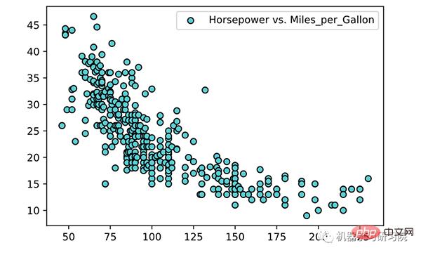
<span style="color: rgb(106, 115, 125); margin: 0px; padding: 0px; background: none 0% 0% / auto repeat scroll padding-box border-box rgba(0, 0, 0, 0);"># 过滤特定列中的NaN行</span><br><span style="color: rgb(89, 89, 89); margin: 0px; padding: 0px; background: none 0% 0% / auto repeat scroll padding-box border-box rgba(0, 0, 0, 0);">df</span>.<span style="color: rgb(0, 92, 197); margin: 0px; padding: 0px; background: none 0% 0% / auto repeat scroll padding-box border-box rgba(0, 0, 0, 0);">dropna</span>(<span style="color: rgb(89, 89, 89); margin: 0px; padding: 0px; background: none 0% 0% / auto repeat scroll padding-box border-box rgba(0, 0, 0, 0);">subset</span><span style="color: rgb(215, 58, 73); margin: 0px; padding: 0px; background: none 0% 0% / auto repeat scroll padding-box border-box rgba(0, 0, 0, 0);">=</span>[<span style="color: rgb(102, 153, 0); margin: 0px; padding: 0px; background: none 0% 0% / auto repeat scroll padding-box border-box rgba(0, 0, 0, 0);">'Horsepower'</span>, <span style="color: rgb(102, 153, 0); margin: 0px; padding: 0px; background: none 0% 0% / auto repeat scroll padding-box border-box rgba(0, 0, 0, 0);">'Miles_per_Gallon'</span>], <span style="color: rgb(89, 89, 89); margin: 0px; padding: 0px; background: none 0% 0% / auto repeat scroll padding-box border-box rgba(0, 0, 0, 0);">inplace</span><span style="color: rgb(215, 58, 73); margin: 0px; padding: 0px; background: none 0% 0% / auto repeat scroll padding-box border-box rgba(0, 0, 0, 0);">=</span><span style="color: rgb(215, 58, 73); margin: 0px; padding: 0px; background: none 0% 0% / auto repeat scroll padding-box border-box rgba(0, 0, 0, 0);">True</span>)<br><span style="color: rgb(89, 89, 89); margin: 0px; padding: 0px; background: none 0% 0% / auto repeat scroll padding-box border-box rgba(0, 0, 0, 0);">df</span>.<span style="color: rgb(0, 92, 197); margin: 0px; padding: 0px; background: none 0% 0% / auto repeat scroll padding-box border-box rgba(0, 0, 0, 0);">sort_values</span>(<span style="color: rgb(89, 89, 89); margin: 0px; padding: 0px; background: none 0% 0% / auto repeat scroll padding-box border-box rgba(0, 0, 0, 0);">by</span><span style="color: rgb(215, 58, 73); margin: 0px; padding: 0px; background: none 0% 0% / auto repeat scroll padding-box border-box rgba(0, 0, 0, 0);">=</span><span style="color: rgb(102, 153, 0); margin: 0px; padding: 0px; background: none 0% 0% / auto repeat scroll padding-box border-box rgba(0, 0, 0, 0);">'Horsepower'</span>, <span style="color: rgb(89, 89, 89); margin: 0px; padding: 0px; background: none 0% 0% / auto repeat scroll padding-box border-box rgba(0, 0, 0, 0);">inplace</span><span style="color: rgb(215, 58, 73); margin: 0px; padding: 0px; background: none 0% 0% / auto repeat scroll padding-box border-box rgba(0, 0, 0, 0);">=</span><span style="color: rgb(215, 58, 73); margin: 0px; padding: 0px; background: none 0% 0% / auto repeat scroll padding-box border-box rgba(0, 0, 0, 0);">True</span>)<br><span style="color: rgb(106, 115, 125); margin: 0px; padding: 0px; background: none 0% 0% / auto repeat scroll padding-box border-box rgba(0, 0, 0, 0);"># 数据转换</span><br><span style="color: rgb(89, 89, 89); margin: 0px; padding: 0px; background: none 0% 0% / auto repeat scroll padding-box border-box rgba(0, 0, 0, 0);">X</span> <span style="color: rgb(215, 58, 73); margin: 0px; padding: 0px; background: none 0% 0% / auto repeat scroll padding-box border-box rgba(0, 0, 0, 0);">=</span> <span style="color: rgb(89, 89, 89); margin: 0px; padding: 0px; background: none 0% 0% / auto repeat scroll padding-box border-box rgba(0, 0, 0, 0);">df</span>[<span style="color: rgb(102, 153, 0); margin: 0px; padding: 0px; background: none 0% 0% / auto repeat scroll padding-box border-box rgba(0, 0, 0, 0);">'Horsepower'</span>].<span style="color: rgb(0, 92, 197); margin: 0px; padding: 0px; background: none 0% 0% / auto repeat scroll padding-box border-box rgba(0, 0, 0, 0);">to_numpy</span>().<span style="color: rgb(0, 92, 197); margin: 0px; padding: 0px; background: none 0% 0% / auto repeat scroll padding-box border-box rgba(0, 0, 0, 0);">reshape</span>(<span style="color: rgb(215, 58, 73); margin: 0px; padding: 0px; background: none 0% 0% / auto repeat scroll padding-box border-box rgba(0, 0, 0, 0);">-</span><span style="color: rgb(0, 92, 197); margin: 0px; padding: 0px; background: none 0% 0% / auto repeat scroll padding-box border-box rgba(0, 0, 0, 0);">1</span>, <span style="color: rgb(0, 92, 197); margin: 0px; padding: 0px; background: none 0% 0% / auto repeat scroll padding-box border-box rgba(0, 0, 0, 0);">1</span>)<br><span style="color: rgb(89, 89, 89); margin: 0px; padding: 0px; background: none 0% 0% / auto repeat scroll padding-box border-box rgba(0, 0, 0, 0);">y</span> <span style="color: rgb(215, 58, 73); margin: 0px; padding: 0px; background: none 0% 0% / auto repeat scroll padding-box border-box rgba(0, 0, 0, 0);">=</span> <span style="color: rgb(89, 89, 89); margin: 0px; padding: 0px; background: none 0% 0% / auto repeat scroll padding-box border-box rgba(0, 0, 0, 0);">df</span>[<span style="color: rgb(102, 153, 0); margin: 0px; padding: 0px; background: none 0% 0% / auto repeat scroll padding-box border-box rgba(0, 0, 0, 0);">'Miles_per_Gallon'</span>].<span style="color: rgb(0, 92, 197); margin: 0px; padding: 0px; background: none 0% 0% / auto repeat scroll padding-box border-box rgba(0, 0, 0, 0);">to_numpy</span>().<span style="color: rgb(0, 92, 197); margin: 0px; padding: 0px; background: none 0% 0% / auto repeat scroll padding-box border-box rgba(0, 0, 0, 0);">reshape</span>(<span style="color: rgb(215, 58, 73); margin: 0px; padding: 0px; background: none 0% 0% / auto repeat scroll padding-box border-box rgba(0, 0, 0, 0);">-</span><span style="color: rgb(0, 92, 197); margin: 0px; padding: 0px; background: none 0% 0% / auto repeat scroll padding-box border-box rgba(0, 0, 0, 0);">1</span>, <span style="color: rgb(0, 92, 197); margin: 0px; padding: 0px; background: none 0% 0% / auto repeat scroll padding-box border-box rgba(0, 0, 0, 0);">1</span>)<br><span style="color: rgb(89, 89, 89); margin: 0px; padding: 0px; background: none 0% 0% / auto repeat scroll padding-box border-box rgba(0, 0, 0, 0);">plt</span>.<span style="color: rgb(0, 92, 197); margin: 0px; padding: 0px; background: none 0% 0% / auto repeat scroll padding-box border-box rgba(0, 0, 0, 0);">scatter</span>(<span style="color: rgb(89, 89, 89); margin: 0px; padding: 0px; background: none 0% 0% / auto repeat scroll padding-box border-box rgba(0, 0, 0, 0);">X</span>, <span style="color: rgb(89, 89, 89); margin: 0px; padding: 0px; background: none 0% 0% / auto repeat scroll padding-box border-box rgba(0, 0, 0, 0);">y</span>, <span style="color: rgb(89, 89, 89); margin: 0px; padding: 0px; background: none 0% 0% / auto repeat scroll padding-box border-box rgba(0, 0, 0, 0);">color</span><span style="color: rgb(215, 58, 73); margin: 0px; padding: 0px; background: none 0% 0% / auto repeat scroll padding-box border-box rgba(0, 0, 0, 0);">=</span><span style="color: rgb(102, 153, 0); margin: 0px; padding: 0px; background: none 0% 0% / auto repeat scroll padding-box border-box rgba(0, 0, 0, 0);">'teal'</span>, <span style="color: rgb(89, 89, 89); margin: 0px; padding: 0px; background: none 0% 0% / auto repeat scroll padding-box border-box rgba(0, 0, 0, 0);">edgecolors</span><span style="color: rgb(215, 58, 73); margin: 0px; padding: 0px; background: none 0% 0% / auto repeat scroll padding-box border-box rgba(0, 0, 0, 0);">=</span><span style="color: rgb(102, 153, 0); margin: 0px; padding: 0px; background: none 0% 0% / auto repeat scroll padding-box border-box rgba(0, 0, 0, 0);">'black'</span>, <span style="color: rgb(89, 89, 89); margin: 0px; padding: 0px; background: none 0% 0% / auto repeat scroll padding-box border-box rgba(0, 0, 0, 0);">label</span><span style="color: rgb(215, 58, 73); margin: 0px; padding: 0px; background: none 0% 0% / auto repeat scroll padding-box border-box rgba(0, 0, 0, 0);">=</span><span style="color: rgb(102, 153, 0); margin: 0px; padding: 0px; background: none 0% 0% / auto repeat scroll padding-box border-box rgba(0, 0, 0, 0);">'Horsepower vs. Miles_per_Gallon'</span>)<br><span style="color: rgb(89, 89, 89); margin: 0px; padding: 0px; background: none 0% 0% / auto repeat scroll padding-box border-box rgba(0, 0, 0, 0);">plt</span>.<span style="color: rgb(0, 92, 197); margin: 0px; padding: 0px; background: none 0% 0% / auto repeat scroll padding-box border-box rgba(0, 0, 0, 0);">legend</span>()<br><span style="color: rgb(89, 89, 89); margin: 0px; padding: 0px; background: none 0% 0% / auto repeat scroll padding-box border-box rgba(0, 0, 0, 0);">plt</span>.<span style="color: rgb(0, 92, 197); margin: 0px; padding: 0px; background: none 0% 0% / auto repeat scroll padding-box border-box rgba(0, 0, 0, 0);">show</span>()<br>

Copy after login

Summary of nine top-flow regression algorithms and examples

1. Linear Regression

Linear regression is often the first algorithm learned in machine learning and data science. Linear regression is a linear model that assumes a linear relationship between an input variable (X) and a single output variable (y). Generally speaking, there are two situations:

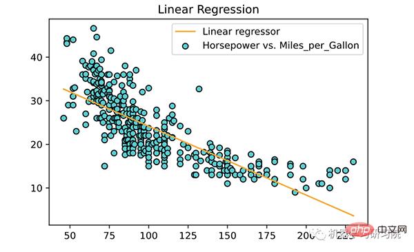
Univariate linear regression: It represents the relationship between a single input variable and a single output variable model.
Multivariable linear regression (also called multiple linear regression): It models the relationship between multiple input variables and a single output variable.

This algorithm is very common. Scikit-learn[2] has a built-in simple linear regression LinearRegression() algorithm. Next, create a LinearRegression object with the little monkey and use the training data for training.

<span style="color: rgb(215, 58, 73); margin: 0px; padding: 0px; background: none 0% 0% / auto repeat scroll padding-box border-box rgba(0, 0, 0, 0);">from</span> <span style="color: rgb(89, 89, 89); margin: 0px; padding: 0px; background: none 0% 0% / auto repeat scroll padding-box border-box rgba(0, 0, 0, 0);">sklearn</span>.<span style="color: rgb(0, 92, 197); margin: 0px; padding: 0px; background: none 0% 0% / auto repeat scroll padding-box border-box rgba(0, 0, 0, 0);">linear_model</span> <span style="color: rgb(215, 58, 73); margin: 0px; padding: 0px; background: none 0% 0% / auto repeat scroll padding-box border-box rgba(0, 0, 0, 0);">import</span> <span style="color: rgb(89, 89, 89); margin: 0px; padding: 0px; background: none 0% 0% / auto repeat scroll padding-box border-box rgba(0, 0, 0, 0);">LinearRegression</span> <span style="color: rgb(106, 115, 125); margin: 0px; padding: 0px; background: none 0% 0% / auto repeat scroll padding-box border-box rgba(0, 0, 0, 0);"># 创建和训练模型</span><br><span style="color: rgb(89, 89, 89); margin: 0px; padding: 0px; background: none 0% 0% / auto repeat scroll padding-box border-box rgba(0, 0, 0, 0);">linear_regressor</span> <span style="color: rgb(215, 58, 73); margin: 0px; padding: 0px; background: none 0% 0% / auto repeat scroll padding-box border-box rgba(0, 0, 0, 0);">=</span> <span style="color: rgb(89, 89, 89); margin: 0px; padding: 0px; background: none 0% 0% / auto repeat scroll padding-box border-box rgba(0, 0, 0, 0);">LinearRegression</span>()<br><span style="color: rgb(89, 89, 89); margin: 0px; padding: 0px; background: none 0% 0% / auto repeat scroll padding-box border-box rgba(0, 0, 0, 0);">linear_regressor</span>.<span style="color: rgb(0, 92, 197); margin: 0px; padding: 0px; background: none 0% 0% / auto repeat scroll padding-box border-box rgba(0, 0, 0, 0);">fit</span>(<span style="color: rgb(89, 89, 89); margin: 0px; padding: 0px; background: none 0% 0% / auto repeat scroll padding-box border-box rgba(0, 0, 0, 0);">X</span>, <span style="color: rgb(89, 89, 89); margin: 0px; padding: 0px; background: none 0% 0% / auto repeat scroll padding-box border-box rgba(0, 0, 0, 0);">y</span>)<br>

Copy after login

After training is completed, you can use the coef_ attribute of LinearRegression to view the model coefficient parameters:

<span style="color: rgb(89, 89, 89); margin: 0px; padding: 0px; background: none 0% 0% / auto repeat scroll padding-box border-box rgba(0, 0, 0, 0);">linear_regressor</span>.<span style="color: rgb(0, 92, 197); margin: 0px; padding: 0px; background: none 0% 0% / auto repeat scroll padding-box border-box rgba(0, 0, 0, 0);">coef_</span><br>

Copy after login

<span style="color: rgb(89, 89, 89); margin: 0px; padding: 0px; background: none 0% 0% / auto repeat scroll padding-box border-box rgba(0, 0, 0, 0);">array</span>([[<span style="color: rgb(215, 58, 73); margin: 0px; padding: 0px; background: none 0% 0% / auto repeat scroll padding-box border-box rgba(0, 0, 0, 0);">-</span><span style="color: rgb(0, 92, 197); margin: 0px; padding: 0px; background: none 0% 0% / auto repeat scroll padding-box border-box rgba(0, 0, 0, 0);">0.15784473</span>]])<br>

Copy after login

Now use the trained model and fit a line to the training data.

<span style="color: rgb(106, 115, 125); margin: 0px; padding: 0px; background: none 0% 0% / auto repeat scroll padding-box border-box rgba(0, 0, 0, 0);"># 为训练数据绘制点和拟合线</span><br><span style="color: rgb(89, 89, 89); margin: 0px; padding: 0px; background: none 0% 0% / auto repeat scroll padding-box border-box rgba(0, 0, 0, 0);">plt</span>.<span style="color: rgb(0, 92, 197); margin: 0px; padding: 0px; background: none 0% 0% / auto repeat scroll padding-box border-box rgba(0, 0, 0, 0);">scatter</span>(<span style="color: rgb(89, 89, 89); margin: 0px; padding: 0px; background: none 0% 0% / auto repeat scroll padding-box border-box rgba(0, 0, 0, 0);">X</span>, <span style="color: rgb(89, 89, 89); margin: 0px; padding: 0px; background: none 0% 0% / auto repeat scroll padding-box border-box rgba(0, 0, 0, 0);">y</span>, <span style="color: rgb(89, 89, 89); margin: 0px; padding: 0px; background: none 0% 0% / auto repeat scroll padding-box border-box rgba(0, 0, 0, 0);">color</span><span style="color: rgb(215, 58, 73); margin: 0px; padding: 0px; background: none 0% 0% / auto repeat scroll padding-box border-box rgba(0, 0, 0, 0);">=</span><span style="color: rgb(102, 153, 0); margin: 0px; padding: 0px; background: none 0% 0% / auto repeat scroll padding-box border-box rgba(0, 0, 0, 0);">'RoyalBlue'</span>, <span style="color: rgb(89, 89, 89); margin: 0px; padding: 0px; background: none 0% 0% / auto repeat scroll padding-box border-box rgba(0, 0, 0, 0);">edgecolors</span><span style="color: rgb(215, 58, 73); margin: 0px; padding: 0px; background: none 0% 0% / auto repeat scroll padding-box border-box rgba(0, 0, 0, 0);">=</span><span style="color: rgb(102, 153, 0); margin: 0px; padding: 0px; background: none 0% 0% / auto repeat scroll padding-box border-box rgba(0, 0, 0, 0);">'black'</span>, <span style="color: rgb(89, 89, 89); margin: 0px; padding: 0px; background: none 0% 0% / auto repeat scroll padding-box border-box rgba(0, 0, 0, 0);">label</span><span style="color: rgb(215, 58, 73); margin: 0px; padding: 0px; background: none 0% 0% / auto repeat scroll padding-box border-box rgba(0, 0, 0, 0);">=</span><span style="color: rgb(102, 153, 0); margin: 0px; padding: 0px; background: none 0% 0% / auto repeat scroll padding-box border-box rgba(0, 0, 0, 0);">'Horsepower vs. Miles_per_Gallon'</span>)<br><span style="color: rgb(89, 89, 89); margin: 0px; padding: 0px; background: none 0% 0% / auto repeat scroll padding-box border-box rgba(0, 0, 0, 0);">plt</span>.<span style="color: rgb(0, 92, 197); margin: 0px; padding: 0px; background: none 0% 0% / auto repeat scroll padding-box border-box rgba(0, 0, 0, 0);">plot</span>(<span style="color: rgb(89, 89, 89); margin: 0px; padding: 0px; background: none 0% 0% / auto repeat scroll padding-box border-box rgba(0, 0, 0, 0);">X</span>, <span style="color: rgb(89, 89, 89); margin: 0px; padding: 0px; background: none 0% 0% / auto repeat scroll padding-box border-box rgba(0, 0, 0, 0);">linear_regressor</span>.<span style="color: rgb(0, 92, 197); margin: 0px; padding: 0px; background: none 0% 0% / auto repeat scroll padding-box border-box rgba(0, 0, 0, 0);">predict</span>(<span style="color: rgb(89, 89, 89); margin: 0px; padding: 0px; background: none 0% 0% / auto repeat scroll padding-box border-box rgba(0, 0, 0, 0);">X</span>), <span style="color: rgb(89, 89, 89); margin: 0px; padding: 0px; background: none 0% 0% / auto repeat scroll padding-box border-box rgba(0, 0, 0, 0);">color</span><span style="color: rgb(215, 58, 73); margin: 0px; padding: 0px; background: none 0% 0% / auto repeat scroll padding-box border-box rgba(0, 0, 0, 0);">=</span><span style="color: rgb(102, 153, 0); margin: 0px; padding: 0px; background: none 0% 0% / auto repeat scroll padding-box border-box rgba(0, 0, 0, 0);">'orange'</span>, <span style="color: rgb(89, 89, 89); margin: 0px; padding: 0px; background: none 0% 0% / auto repeat scroll padding-box border-box rgba(0, 0, 0, 0);">label</span><span style="color: rgb(215, 58, 73); margin: 0px; padding: 0px; background: none 0% 0% / auto repeat scroll padding-box border-box rgba(0, 0, 0, 0);">=</span><span style="color: rgb(102, 153, 0); margin: 0px; padding: 0px; background: none 0% 0% / auto repeat scroll padding-box border-box rgba(0, 0, 0, 0);">'Linear regressor'</span>)<br><span style="color: rgb(89, 89, 89); margin: 0px; padding: 0px; background: none 0% 0% / auto repeat scroll padding-box border-box rgba(0, 0, 0, 0);">plt</span>.<span style="color: rgb(0, 92, 197); margin: 0px; padding: 0px; background: none 0% 0% / auto repeat scroll padding-box border-box rgba(0, 0, 0, 0);">title</span>(<span style="color: rgb(102, 153, 0); margin: 0px; padding: 0px; background: none 0% 0% / auto repeat scroll padding-box border-box rgba(0, 0, 0, 0);">'Linear Regression'</span>)<br><span style="color: rgb(89, 89, 89); margin: 0px; padding: 0px; background: none 0% 0% / auto repeat scroll padding-box border-box rgba(0, 0, 0, 0);">plt</span>.<span style="color: rgb(0, 92, 197); margin: 0px; padding: 0px; background: none 0% 0% / auto repeat scroll padding-box border-box rgba(0, 0, 0, 0);">legend</span>()<br><span style="color: rgb(89, 89, 89); margin: 0px; padding: 0px; background: none 0% 0% / auto repeat scroll padding-box border-box rgba(0, 0, 0, 0);">plt</span>.<span style="color: rgb(0, 92, 197); margin: 0px; padding: 0px; background: none 0% 0% / auto repeat scroll padding-box border-box rgba(0, 0, 0, 0);">show</span>()<br>

Copy after login

Summary of nine top-flow regression algorithms and examples

Summary

A few key points about linear regression:

Fast and easy to model
Linear regression is particularly useful when the relationship to be modeled is not very complex and there is not a large amount of data.
Very intuitive understanding and explanation.
It is very sensitive to outliers.

2. Polynomial Regression

Polynomial regression is one of the most popular choices when you want to create a model for nonlinear separable data. It is similar to linear regression but uses the relationship between variables X and y and finds the best way to draw a fit curve for the data points.

For polynomial regression, some independent variables have powers greater than 1. For example, one might propose the following quadratic model:

β_0, β_1, and β_2 are coefficients
x is a variable/feature
ε is the residual

Scikit-learn has built-in polynomial regression PolynomialFeatures. First, we need to generate a feature matrix consisting of all polynomial features with a specified degree:

<span style="color: rgb(215, 58, 73); margin: 0px; padding: 0px; background: none 0% 0% / auto repeat scroll padding-box border-box rgba(0, 0, 0, 0);">from</span> <span style="color: rgb(89, 89, 89); margin: 0px; padding: 0px; background: none 0% 0% / auto repeat scroll padding-box border-box rgba(0, 0, 0, 0);">sklearn</span>.<span style="color: rgb(0, 92, 197); margin: 0px; padding: 0px; background: none 0% 0% / auto repeat scroll padding-box border-box rgba(0, 0, 0, 0);">preprocessing</span> <span style="color: rgb(215, 58, 73); margin: 0px; padding: 0px; background: none 0% 0% / auto repeat scroll padding-box border-box rgba(0, 0, 0, 0);">import</span> <span style="color: rgb(89, 89, 89); margin: 0px; padding: 0px; background: none 0% 0% / auto repeat scroll padding-box border-box rgba(0, 0, 0, 0);">PolynomialFeatures</span><br><span style="color: rgb(106, 115, 125); margin: 0px; padding: 0px; background: none 0% 0% / auto repeat scroll padding-box border-box rgba(0, 0, 0, 0);"># 为二次模型生成矩阵</span><br><span style="color: rgb(106, 115, 125); margin: 0px; padding: 0px; background: none 0% 0% / auto repeat scroll padding-box border-box rgba(0, 0, 0, 0);"># 这里只是简单地生成X^0 X^1和X^2的矩阵</span><br><span style="color: rgb(89, 89, 89); margin: 0px; padding: 0px; background: none 0% 0% / auto repeat scroll padding-box border-box rgba(0, 0, 0, 0);">poly_reg</span> <span style="color: rgb(215, 58, 73); margin: 0px; padding: 0px; background: none 0% 0% / auto repeat scroll padding-box border-box rgba(0, 0, 0, 0);">=</span> <span style="color: rgb(89, 89, 89); margin: 0px; padding: 0px; background: none 0% 0% / auto repeat scroll padding-box border-box rgba(0, 0, 0, 0);">PolynomialFeatures</span>(<span style="color: rgb(89, 89, 89); margin: 0px; padding: 0px; background: none 0% 0% / auto repeat scroll padding-box border-box rgba(0, 0, 0, 0);">degree</span> <span style="color: rgb(215, 58, 73); margin: 0px; padding: 0px; background: none 0% 0% / auto repeat scroll padding-box border-box rgba(0, 0, 0, 0);">=</span> <span style="color: rgb(0, 92, 197); margin: 0px; padding: 0px; background: none 0% 0% / auto repeat scroll padding-box border-box rgba(0, 0, 0, 0);">2</span> )<br><span style="color: rgb(89, 89, 89); margin: 0px; padding: 0px; background: none 0% 0% / auto repeat scroll padding-box border-box rgba(0, 0, 0, 0);">X_poly</span> <span style="color: rgb(215, 58, 73); margin: 0px; padding: 0px; background: none 0% 0% / auto repeat scroll padding-box border-box rgba(0, 0, 0, 0);">=</span> <span style="color: rgb(89, 89, 89); margin: 0px; padding: 0px; background: none 0% 0% / auto repeat scroll padding-box border-box rgba(0, 0, 0, 0);">poly_reg</span>.<span style="color: rgb(0, 92, 197); margin: 0px; padding: 0px; background: none 0% 0% / auto repeat scroll padding-box border-box rgba(0, 0, 0, 0);">fit_transform</span>(<span style="color: rgb(89, 89, 89); margin: 0px; padding: 0px; background: none 0% 0% / auto repeat scroll padding-box border-box rgba(0, 0, 0, 0);">X</span>)<br>

Copy after login

Next, let’s create a LinearRegression object and fit it to the X_poly feature matrix we just generated.

<span style="color: rgb(106, 115, 125); margin: 0px; padding: 0px; background: none 0% 0% / auto repeat scroll padding-box border-box rgba(0, 0, 0, 0);"># 多项式回归模型</span><br><span style="color: rgb(89, 89, 89); margin: 0px; padding: 0px; background: none 0% 0% / auto repeat scroll padding-box border-box rgba(0, 0, 0, 0);">poly_reg_model</span> <span style="color: rgb(215, 58, 73); margin: 0px; padding: 0px; background: none 0% 0% / auto repeat scroll padding-box border-box rgba(0, 0, 0, 0);">=</span> <span style="color: rgb(89, 89, 89); margin: 0px; padding: 0px; background: none 0% 0% / auto repeat scroll padding-box border-box rgba(0, 0, 0, 0);">LinearRegression</span>()<br><span style="color: rgb(89, 89, 89); margin: 0px; padding: 0px; background: none 0% 0% / auto repeat scroll padding-box border-box rgba(0, 0, 0, 0);">poly_reg_model</span>.<span style="color: rgb(0, 92, 197); margin: 0px; padding: 0px; background: none 0% 0% / auto repeat scroll padding-box border-box rgba(0, 0, 0, 0);">fit</span>(<span style="color: rgb(89, 89, 89); margin: 0px; padding: 0px; background: none 0% 0% / auto repeat scroll padding-box border-box rgba(0, 0, 0, 0);">X_poly</span>, <span style="color: rgb(89, 89, 89); margin: 0px; padding: 0px; background: none 0% 0% / auto repeat scroll padding-box border-box rgba(0, 0, 0, 0);">y</span>)<br>

Copy after login

Now take the model and fit a line to the training data, the X_plot looks like this:

<span style="color: rgb(106, 115, 125); margin: 0px; padding: 0px; background: none 0% 0% / auto repeat scroll padding-box border-box rgba(0, 0, 0, 0);"># 为训练数据绘制点和拟合线</span><br><span style="color: rgb(89, 89, 89); margin: 0px; padding: 0px; background: none 0% 0% / auto repeat scroll padding-box border-box rgba(0, 0, 0, 0);">plt</span>.<span style="color: rgb(0, 92, 197); margin: 0px; padding: 0px; background: none 0% 0% / auto repeat scroll padding-box border-box rgba(0, 0, 0, 0);">scatter</span>(<span style="color: rgb(89, 89, 89); margin: 0px; padding: 0px; background: none 0% 0% / auto repeat scroll padding-box border-box rgba(0, 0, 0, 0);">X</span>, <span style="color: rgb(89, 89, 89); margin: 0px; padding: 0px; background: none 0% 0% / auto repeat scroll padding-box border-box rgba(0, 0, 0, 0);">y</span>, <span style="color: rgb(89, 89, 89); margin: 0px; padding: 0px; background: none 0% 0% / auto repeat scroll padding-box border-box rgba(0, 0, 0, 0);">color</span><span style="color: rgb(215, 58, 73); margin: 0px; padding: 0px; background: none 0% 0% / auto repeat scroll padding-box border-box rgba(0, 0, 0, 0);">=</span><span style="color: rgb(102, 153, 0); margin: 0px; padding: 0px; background: none 0% 0% / auto repeat scroll padding-box border-box rgba(0, 0, 0, 0);">'DarkTurquoise'</span>, <span style="color: rgb(89, 89, 89); margin: 0px; padding: 0px; background: none 0% 0% / auto repeat scroll padding-box border-box rgba(0, 0, 0, 0);">edgecolors</span><span style="color: rgb(215, 58, 73); margin: 0px; padding: 0px; background: none 0% 0% / auto repeat scroll padding-box border-box rgba(0, 0, 0, 0);">=</span><span style="color: rgb(102, 153, 0); margin: 0px; padding: 0px; background: none 0% 0% / auto repeat scroll padding-box border-box rgba(0, 0, 0, 0);">'black'</span>,<br><span style="color: rgb(89, 89, 89); margin: 0px; padding: 0px; background: none 0% 0% / auto repeat scroll padding-box border-box rgba(0, 0, 0, 0);">label</span><span style="color: rgb(215, 58, 73); margin: 0px; padding: 0px; background: none 0% 0% / auto repeat scroll padding-box border-box rgba(0, 0, 0, 0);">=</span><span style="color: rgb(102, 153, 0); margin: 0px; padding: 0px; background: none 0% 0% / auto repeat scroll padding-box border-box rgba(0, 0, 0, 0);">'Horsepower vs. Miles_per_Gallon'</span>)<br><span style="color: rgb(89, 89, 89); margin: 0px; padding: 0px; background: none 0% 0% / auto repeat scroll padding-box border-box rgba(0, 0, 0, 0);">plt</span>.<span style="color: rgb(0, 92, 197); margin: 0px; padding: 0px; background: none 0% 0% / auto repeat scroll padding-box border-box rgba(0, 0, 0, 0);">plot</span>(<span style="color: rgb(89, 89, 89); margin: 0px; padding: 0px; background: none 0% 0% / auto repeat scroll padding-box border-box rgba(0, 0, 0, 0);">X</span>, <span style="color: rgb(89, 89, 89); margin: 0px; padding: 0px; background: none 0% 0% / auto repeat scroll padding-box border-box rgba(0, 0, 0, 0);">poly_reg_model</span>.<span style="color: rgb(0, 92, 197); margin: 0px; padding: 0px; background: none 0% 0% / auto repeat scroll padding-box border-box rgba(0, 0, 0, 0);">predict</span>(<span style="color: rgb(89, 89, 89); margin: 0px; padding: 0px; background: none 0% 0% / auto repeat scroll padding-box border-box rgba(0, 0, 0, 0);">X_poly</span>), <span style="color: rgb(89, 89, 89); margin: 0px; padding: 0px; background: none 0% 0% / auto repeat scroll padding-box border-box rgba(0, 0, 0, 0);">color</span><span style="color: rgb(215, 58, 73); margin: 0px; padding: 0px; background: none 0% 0% / auto repeat scroll padding-box border-box rgba(0, 0, 0, 0);">=</span><span style="color: rgb(102, 153, 0); margin: 0px; padding: 0px; background: none 0% 0% / auto repeat scroll padding-box border-box rgba(0, 0, 0, 0);">'orange'</span>,<br> <span style="color: rgb(89, 89, 89); margin: 0px; padding: 0px; background: none 0% 0% / auto repeat scroll padding-box border-box rgba(0, 0, 0, 0);">label</span><span style="color: rgb(215, 58, 73); margin: 0px; padding: 0px; background: none 0% 0% / auto repeat scroll padding-box border-box rgba(0, 0, 0, 0);">=</span><span style="color: rgb(102, 153, 0); margin: 0px; padding: 0px; background: none 0% 0% / auto repeat scroll padding-box border-box rgba(0, 0, 0, 0);">'Polynmial regressor'</span>)<br><span style="color: rgb(89, 89, 89); margin: 0px; padding: 0px; background: none 0% 0% / auto repeat scroll padding-box border-box rgba(0, 0, 0, 0);">plt</span>.<span style="color: rgb(0, 92, 197); margin: 0px; padding: 0px; background: none 0% 0% / auto repeat scroll padding-box border-box rgba(0, 0, 0, 0);">title</span>(<span style="color: rgb(102, 153, 0); margin: 0px; padding: 0px; background: none 0% 0% / auto repeat scroll padding-box border-box rgba(0, 0, 0, 0);">'Polynomial Regression'</span>)<br><span style="color: rgb(89, 89, 89); margin: 0px; padding: 0px; background: none 0% 0% / auto repeat scroll padding-box border-box rgba(0, 0, 0, 0);">plt</span>.<span style="color: rgb(0, 92, 197); margin: 0px; padding: 0px; background: none 0% 0% / auto repeat scroll padding-box border-box rgba(0, 0, 0, 0);">legend</span>()<br><span style="color: rgb(89, 89, 89); margin: 0px; padding: 0px; background: none 0% 0% / auto repeat scroll padding-box border-box rgba(0, 0, 0, 0);">plt</span>.<span style="color: rgb(0, 92, 197); margin: 0px; padding: 0px; background: none 0% 0% / auto repeat scroll padding-box border-box rgba(0, 0, 0, 0);">show</span>()<br>

Copy after login

Summary of nine top-flow regression algorithms and examples

Summary

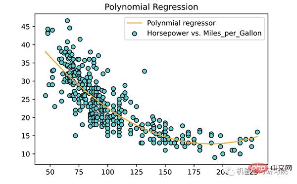
About polynomials Several key points of return:

能够对非线性可分数据进行建模；而线性回归不能做到这一点。它总体上更加灵活，可以对一些相当复杂的关系进行建模。
完全控制特征变量的建模（可指定设置指数）。
需要精心设计，需要一些数据知识才能选择最佳指数。
如果指数选择不当，则容易过度拟合。

3. 支持向量回归

众所周知的支持向量机在处理分类问题时非常有效。其实，SVM 也经常用在回归问题中，被称为支持向量回归(SVR)。同样，Scikit-learn内置了这种方法SVR()。

在拟合 SVR 模型之前，通常较好的做法是对数据进行数据标准化操作，及对特征进行缩放。数据标准化的目的是为了确保每个特征都具有相似的重要性。我们通过StandardScaler()方法对训练数据操作。

<span style="color: rgb(215, 58, 73); margin: 0px; padding: 0px; background: none 0% 0% / auto repeat scroll padding-box border-box rgba(0, 0, 0, 0);">from</span> <span style="color: rgb(89, 89, 89); margin: 0px; padding: 0px; background: none 0% 0% / auto repeat scroll padding-box border-box rgba(0, 0, 0, 0);">sklearn</span>.<span style="color: rgb(0, 92, 197); margin: 0px; padding: 0px; background: none 0% 0% / auto repeat scroll padding-box border-box rgba(0, 0, 0, 0);">svm</span> <span style="color: rgb(215, 58, 73); margin: 0px; padding: 0px; background: none 0% 0% / auto repeat scroll padding-box border-box rgba(0, 0, 0, 0);">import</span> <span style="color: rgb(89, 89, 89); margin: 0px; padding: 0px; background: none 0% 0% / auto repeat scroll padding-box border-box rgba(0, 0, 0, 0);">SVR</span><br><span style="color: rgb(215, 58, 73); margin: 0px; padding: 0px; background: none 0% 0% / auto repeat scroll padding-box border-box rgba(0, 0, 0, 0);">from</span> <span style="color: rgb(89, 89, 89); margin: 0px; padding: 0px; background: none 0% 0% / auto repeat scroll padding-box border-box rgba(0, 0, 0, 0);">sklearn</span>.<span style="color: rgb(0, 92, 197); margin: 0px; padding: 0px; background: none 0% 0% / auto repeat scroll padding-box border-box rgba(0, 0, 0, 0);">preprocessing</span> <span style="color: rgb(215, 58, 73); margin: 0px; padding: 0px; background: none 0% 0% / auto repeat scroll padding-box border-box rgba(0, 0, 0, 0);">import</span> <span style="color: rgb(89, 89, 89); margin: 0px; padding: 0px; background: none 0% 0% / auto repeat scroll padding-box border-box rgba(0, 0, 0, 0);">StandardScaler</span> <span style="color: rgb(106, 115, 125); margin: 0px; padding: 0px; background: none 0% 0% / auto repeat scroll padding-box border-box rgba(0, 0, 0, 0);"># 执行特征缩放</span><br><span style="color: rgb(89, 89, 89); margin: 0px; padding: 0px; background: none 0% 0% / auto repeat scroll padding-box border-box rgba(0, 0, 0, 0);">scaled_X</span> <span style="color: rgb(215, 58, 73); margin: 0px; padding: 0px; background: none 0% 0% / auto repeat scroll padding-box border-box rgba(0, 0, 0, 0);">=</span> <span style="color: rgb(89, 89, 89); margin: 0px; padding: 0px; background: none 0% 0% / auto repeat scroll padding-box border-box rgba(0, 0, 0, 0);">StandardScaler</span>()<br><span style="color: rgb(89, 89, 89); margin: 0px; padding: 0px; background: none 0% 0% / auto repeat scroll padding-box border-box rgba(0, 0, 0, 0);">scaled_y</span> <span style="color: rgb(215, 58, 73); margin: 0px; padding: 0px; background: none 0% 0% / auto repeat scroll padding-box border-box rgba(0, 0, 0, 0);">=</span> <span style="color: rgb(89, 89, 89); margin: 0px; padding: 0px; background: none 0% 0% / auto repeat scroll padding-box border-box rgba(0, 0, 0, 0);">StandardScaler</span>()<br><span style="color: rgb(89, 89, 89); margin: 0px; padding: 0px; background: none 0% 0% / auto repeat scroll padding-box border-box rgba(0, 0, 0, 0);">scaled_X</span> <span style="color: rgb(215, 58, 73); margin: 0px; padding: 0px; background: none 0% 0% / auto repeat scroll padding-box border-box rgba(0, 0, 0, 0);">=</span> <span style="color: rgb(89, 89, 89); margin: 0px; padding: 0px; background: none 0% 0% / auto repeat scroll padding-box border-box rgba(0, 0, 0, 0);">scaled_X</span>.<span style="color: rgb(0, 92, 197); margin: 0px; padding: 0px; background: none 0% 0% / auto repeat scroll padding-box border-box rgba(0, 0, 0, 0);">fit_transform</span>(<span style="color: rgb(89, 89, 89); margin: 0px; padding: 0px; background: none 0% 0% / auto repeat scroll padding-box border-box rgba(0, 0, 0, 0);">X</span>)<br><span style="color: rgb(89, 89, 89); margin: 0px; padding: 0px; background: none 0% 0% / auto repeat scroll padding-box border-box rgba(0, 0, 0, 0);">scaled_y</span> <span style="color: rgb(215, 58, 73); margin: 0px; padding: 0px; background: none 0% 0% / auto repeat scroll padding-box border-box rgba(0, 0, 0, 0);">=</span> <span style="color: rgb(89, 89, 89); margin: 0px; padding: 0px; background: none 0% 0% / auto repeat scroll padding-box border-box rgba(0, 0, 0, 0);">scaled_y</span>.<span style="color: rgb(0, 92, 197); margin: 0px; padding: 0px; background: none 0% 0% / auto repeat scroll padding-box border-box rgba(0, 0, 0, 0);">fit_transform</span>(<span style="color: rgb(89, 89, 89); margin: 0px; padding: 0px; background: none 0% 0% / auto repeat scroll padding-box border-box rgba(0, 0, 0, 0);">y</span>)<br>

Copy after login

接下来，我们创建了一个SVR与对象的内核设置为'rbf'和伽玛设置为'auto'。之后，我们调用fit()使其适合缩放的训练数据：

<span style="color: rgb(89, 89, 89); margin: 0px; padding: 0px; background: none 0% 0% / auto repeat scroll padding-box border-box rgba(0, 0, 0, 0);">svr_regressor</span> <span style="color: rgb(215, 58, 73); margin: 0px; padding: 0px; background: none 0% 0% / auto repeat scroll padding-box border-box rgba(0, 0, 0, 0);">=</span> <span style="color: rgb(89, 89, 89); margin: 0px; padding: 0px; background: none 0% 0% / auto repeat scroll padding-box border-box rgba(0, 0, 0, 0);">SVR</span>(<span style="color: rgb(89, 89, 89); margin: 0px; padding: 0px; background: none 0% 0% / auto repeat scroll padding-box border-box rgba(0, 0, 0, 0);">kernel</span><span style="color: rgb(215, 58, 73); margin: 0px; padding: 0px; background: none 0% 0% / auto repeat scroll padding-box border-box rgba(0, 0, 0, 0);">=</span><span style="color: rgb(102, 153, 0); margin: 0px; padding: 0px; background: none 0% 0% / auto repeat scroll padding-box border-box rgba(0, 0, 0, 0);">'rbf'</span>, <span style="color: rgb(89, 89, 89); margin: 0px; padding: 0px; background: none 0% 0% / auto repeat scroll padding-box border-box rgba(0, 0, 0, 0);">gamma</span><span style="color: rgb(215, 58, 73); margin: 0px; padding: 0px; background: none 0% 0% / auto repeat scroll padding-box border-box rgba(0, 0, 0, 0);">=</span><span style="color: rgb(102, 153, 0); margin: 0px; padding: 0px; background: none 0% 0% / auto repeat scroll padding-box border-box rgba(0, 0, 0, 0);">'auto'</span>)<br><span style="color: rgb(89, 89, 89); margin: 0px; padding: 0px; background: none 0% 0% / auto repeat scroll padding-box border-box rgba(0, 0, 0, 0);">svr_regressor</span>.<span style="color: rgb(0, 92, 197); margin: 0px; padding: 0px; background: none 0% 0% / auto repeat scroll padding-box border-box rgba(0, 0, 0, 0);">fit</span>(<span style="color: rgb(89, 89, 89); margin: 0px; padding: 0px; background: none 0% 0% / auto repeat scroll padding-box border-box rgba(0, 0, 0, 0);">scaled_X</span>, <span style="color: rgb(89, 89, 89); margin: 0px; padding: 0px; background: none 0% 0% / auto repeat scroll padding-box border-box rgba(0, 0, 0, 0);">scaled_y</span>.<span style="color: rgb(0, 92, 197); margin: 0px; padding: 0px; background: none 0% 0% / auto repeat scroll padding-box border-box rgba(0, 0, 0, 0);">ravel</span>())<br>

Copy after login

现在采用该模型并为训练数据拟合一条线，scaled_X如下所示：

<span style="color: rgb(89, 89, 89); margin: 0px; padding: 0px; background: none 0% 0% / auto repeat scroll padding-box border-box rgba(0, 0, 0, 0);">plt</span>.<span style="color: rgb(0, 92, 197); margin: 0px; padding: 0px; background: none 0% 0% / auto repeat scroll padding-box border-box rgba(0, 0, 0, 0);">scatter</span>(<span style="color: rgb(89, 89, 89); margin: 0px; padding: 0px; background: none 0% 0% / auto repeat scroll padding-box border-box rgba(0, 0, 0, 0);">scaled_X</span>, <span style="color: rgb(89, 89, 89); margin: 0px; padding: 0px; background: none 0% 0% / auto repeat scroll padding-box border-box rgba(0, 0, 0, 0);">scaled_y</span>, <span style="color: rgb(89, 89, 89); margin: 0px; padding: 0px; background: none 0% 0% / auto repeat scroll padding-box border-box rgba(0, 0, 0, 0);">color</span><span style="color: rgb(215, 58, 73); margin: 0px; padding: 0px; background: none 0% 0% / auto repeat scroll padding-box border-box rgba(0, 0, 0, 0);">=</span><span style="color: rgb(102, 153, 0); margin: 0px; padding: 0px; background: none 0% 0% / auto repeat scroll padding-box border-box rgba(0, 0, 0, 0);">'DarkTurquoise'</span>,<br><span style="color: rgb(89, 89, 89); margin: 0px; padding: 0px; background: none 0% 0% / auto repeat scroll padding-box border-box rgba(0, 0, 0, 0);">edgecolors</span><span style="color: rgb(215, 58, 73); margin: 0px; padding: 0px; background: none 0% 0% / auto repeat scroll padding-box border-box rgba(0, 0, 0, 0);">=</span><span style="color: rgb(102, 153, 0); margin: 0px; padding: 0px; background: none 0% 0% / auto repeat scroll padding-box border-box rgba(0, 0, 0, 0);">'black'</span>, <span style="color: rgb(89, 89, 89); margin: 0px; padding: 0px; background: none 0% 0% / auto repeat scroll padding-box border-box rgba(0, 0, 0, 0);">label</span><span style="color: rgb(215, 58, 73); margin: 0px; padding: 0px; background: none 0% 0% / auto repeat scroll padding-box border-box rgba(0, 0, 0, 0);">=</span><span style="color: rgb(102, 153, 0); margin: 0px; padding: 0px; background: none 0% 0% / auto repeat scroll padding-box border-box rgba(0, 0, 0, 0);">'Train'</span>)<br><span style="color: rgb(89, 89, 89); margin: 0px; padding: 0px; background: none 0% 0% / auto repeat scroll padding-box border-box rgba(0, 0, 0, 0);">plt</span>.<span style="color: rgb(0, 92, 197); margin: 0px; padding: 0px; background: none 0% 0% / auto repeat scroll padding-box border-box rgba(0, 0, 0, 0);">plot</span>(<span style="color: rgb(89, 89, 89); margin: 0px; padding: 0px; background: none 0% 0% / auto repeat scroll padding-box border-box rgba(0, 0, 0, 0);">scaled_X</span>, <span style="color: rgb(89, 89, 89); margin: 0px; padding: 0px; background: none 0% 0% / auto repeat scroll padding-box border-box rgba(0, 0, 0, 0);">svr_regressor</span>.<span style="color: rgb(0, 92, 197); margin: 0px; padding: 0px; background: none 0% 0% / auto repeat scroll padding-box border-box rgba(0, 0, 0, 0);">predict</span>(<span style="color: rgb(89, 89, 89); margin: 0px; padding: 0px; background: none 0% 0% / auto repeat scroll padding-box border-box rgba(0, 0, 0, 0);">scaled_X</span>),<br> <span style="color: rgb(89, 89, 89); margin: 0px; padding: 0px; background: none 0% 0% / auto repeat scroll padding-box border-box rgba(0, 0, 0, 0);">color</span><span style="color: rgb(215, 58, 73); margin: 0px; padding: 0px; background: none 0% 0% / auto repeat scroll padding-box border-box rgba(0, 0, 0, 0);">=</span><span style="color: rgb(102, 153, 0); margin: 0px; padding: 0px; background: none 0% 0% / auto repeat scroll padding-box border-box rgba(0, 0, 0, 0);">'orange'</span>, <span style="color: rgb(89, 89, 89); margin: 0px; padding: 0px; background: none 0% 0% / auto repeat scroll padding-box border-box rgba(0, 0, 0, 0);">label</span><span style="color: rgb(215, 58, 73); margin: 0px; padding: 0px; background: none 0% 0% / auto repeat scroll padding-box border-box rgba(0, 0, 0, 0);">=</span><span style="color: rgb(102, 153, 0); margin: 0px; padding: 0px; background: none 0% 0% / auto repeat scroll padding-box border-box rgba(0, 0, 0, 0);">'SVR'</span>)<br><span style="color: rgb(89, 89, 89); margin: 0px; padding: 0px; background: none 0% 0% / auto repeat scroll padding-box border-box rgba(0, 0, 0, 0);">plt</span>.<span style="color: rgb(0, 92, 197); margin: 0px; padding: 0px; background: none 0% 0% / auto repeat scroll padding-box border-box rgba(0, 0, 0, 0);">title</span>(<span style="color: rgb(102, 153, 0); margin: 0px; padding: 0px; background: none 0% 0% / auto repeat scroll padding-box border-box rgba(0, 0, 0, 0);">'Simple Vector Regression'</span>)<br><span style="color: rgb(89, 89, 89); margin: 0px; padding: 0px; background: none 0% 0% / auto repeat scroll padding-box border-box rgba(0, 0, 0, 0);">plt</span>.<span style="color: rgb(0, 92, 197); margin: 0px; padding: 0px; background: none 0% 0% / auto repeat scroll padding-box border-box rgba(0, 0, 0, 0);">legend</span>()<br><span style="color: rgb(89, 89, 89); margin: 0px; padding: 0px; background: none 0% 0% / auto repeat scroll padding-box border-box rgba(0, 0, 0, 0);">plt</span>.<span style="color: rgb(0, 92, 197); margin: 0px; padding: 0px; background: none 0% 0% / auto repeat scroll padding-box border-box rgba(0, 0, 0, 0);">show</span>()<br>

Copy after login

Summary of nine top-flow regression algorithms and examples

小结

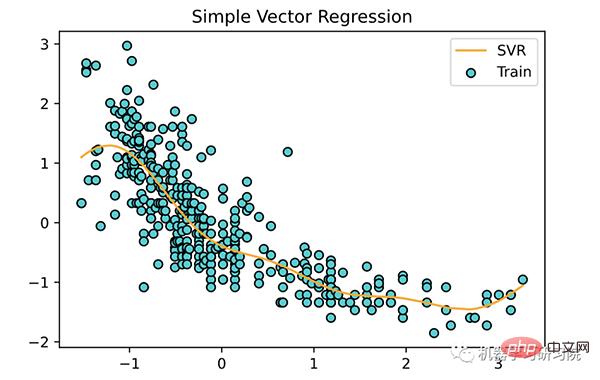
支持向量回归的几个关键点

它对异常值具有鲁棒性并且在高维空间中有效
它具有出色的泛化能力（能够正确适应新的、以前看不见的数据）
如果特征数量远大于样本数量，则容易过拟合

4. 决策树回归

决策树 (DT) 是一种用于分类和回归的非参数监督学习方法。目标是创建一个树模型，通过学习从数据特征推断出的简单决策规则来预测目标变量的值。一棵树可以看作是分段常数近似。

决策树回归也很常见，以至于Scikit-learn内置了DecisionTreeRegressor. 甲DecisionTreeRegressor对象可以在没有特征缩放如下创建：

<span style="color: rgb(215, 58, 73); margin: 0px; padding: 0px; background: none 0% 0% / auto repeat scroll padding-box border-box rgba(0, 0, 0, 0);">from</span> <span style="color: rgb(89, 89, 89); margin: 0px; padding: 0px; background: none 0% 0% / auto repeat scroll padding-box border-box rgba(0, 0, 0, 0);">sklearn</span>.<span style="color: rgb(0, 92, 197); margin: 0px; padding: 0px; background: none 0% 0% / auto repeat scroll padding-box border-box rgba(0, 0, 0, 0);">tree</span> <span style="color: rgb(215, 58, 73); margin: 0px; padding: 0px; background: none 0% 0% / auto repeat scroll padding-box border-box rgba(0, 0, 0, 0);">import</span> <span style="color: rgb(89, 89, 89); margin: 0px; padding: 0px; background: none 0% 0% / auto repeat scroll padding-box border-box rgba(0, 0, 0, 0);">DecisionTreeRegressor</span><br><span style="color: rgb(106, 115, 125); margin: 0px; padding: 0px; background: none 0% 0% / auto repeat scroll padding-box border-box rgba(0, 0, 0, 0);"># 不需要进行特性缩放，因为它将自己处理。</span><br><span style="color: rgb(89, 89, 89); margin: 0px; padding: 0px; background: none 0% 0% / auto repeat scroll padding-box border-box rgba(0, 0, 0, 0);">tree_regressor</span> <span style="color: rgb(215, 58, 73); margin: 0px; padding: 0px; background: none 0% 0% / auto repeat scroll padding-box border-box rgba(0, 0, 0, 0);">=</span> <span style="color: rgb(89, 89, 89); margin: 0px; padding: 0px; background: none 0% 0% / auto repeat scroll padding-box border-box rgba(0, 0, 0, 0);">DecisionTreeRegressor</span>(<span style="color: rgb(89, 89, 89); margin: 0px; padding: 0px; background: none 0% 0% / auto repeat scroll padding-box border-box rgba(0, 0, 0, 0);">random_state</span> <span style="color: rgb(215, 58, 73); margin: 0px; padding: 0px; background: none 0% 0% / auto repeat scroll padding-box border-box rgba(0, 0, 0, 0);">=</span> <span style="color: rgb(0, 92, 197); margin: 0px; padding: 0px; background: none 0% 0% / auto repeat scroll padding-box border-box rgba(0, 0, 0, 0);">0</span>)<br><span style="color: rgb(89, 89, 89); margin: 0px; padding: 0px; background: none 0% 0% / auto repeat scroll padding-box border-box rgba(0, 0, 0, 0);">tree_regressor</span>.<span style="color: rgb(0, 92, 197); margin: 0px; padding: 0px; background: none 0% 0% / auto repeat scroll padding-box border-box rgba(0, 0, 0, 0);">fit</span>(<span style="color: rgb(89, 89, 89); margin: 0px; padding: 0px; background: none 0% 0% / auto repeat scroll padding-box border-box rgba(0, 0, 0, 0);">X</span>, <span style="color: rgb(89, 89, 89); margin: 0px; padding: 0px; background: none 0% 0% / auto repeat scroll padding-box border-box rgba(0, 0, 0, 0);">y</span>)<br>

Copy after login

下面使用训练好的模型，绘制一条拟合曲线。

<span style="color: rgb(89, 89, 89); margin: 0px; padding: 0px; background: none 0% 0% / auto repeat scroll padding-box border-box rgba(0, 0, 0, 0);">X_grid</span> <span style="color: rgb(215, 58, 73); margin: 0px; padding: 0px; background: none 0% 0% / auto repeat scroll padding-box border-box rgba(0, 0, 0, 0);">=</span> <span style="color: rgb(89, 89, 89); margin: 0px; padding: 0px; background: none 0% 0% / auto repeat scroll padding-box border-box rgba(0, 0, 0, 0);">np</span>.<span style="color: rgb(0, 92, 197); margin: 0px; padding: 0px; background: none 0% 0% / auto repeat scroll padding-box border-box rgba(0, 0, 0, 0);">arange</span>(<span style="color: rgb(111, 66, 193); margin: 0px; padding: 0px; background: none 0% 0% / auto repeat scroll padding-box border-box rgba(0, 0, 0, 0);">min</span>(<span style="color: rgb(89, 89, 89); margin: 0px; padding: 0px; background: none 0% 0% / auto repeat scroll padding-box border-box rgba(0, 0, 0, 0);">X</span>), <span style="color: rgb(111, 66, 193); margin: 0px; padding: 0px; background: none 0% 0% / auto repeat scroll padding-box border-box rgba(0, 0, 0, 0);">max</span>(<span style="color: rgb(89, 89, 89); margin: 0px; padding: 0px; background: none 0% 0% / auto repeat scroll padding-box border-box rgba(0, 0, 0, 0);">X</span>), <span style="color: rgb(0, 92, 197); margin: 0px; padding: 0px; background: none 0% 0% / auto repeat scroll padding-box border-box rgba(0, 0, 0, 0);">0.01</span>)<br><span style="color: rgb(89, 89, 89); margin: 0px; padding: 0px; background: none 0% 0% / auto repeat scroll padding-box border-box rgba(0, 0, 0, 0);">X_grid</span> <span style="color: rgb(215, 58, 73); margin: 0px; padding: 0px; background: none 0% 0% / auto repeat scroll padding-box border-box rgba(0, 0, 0, 0);">=</span> <span style="color: rgb(89, 89, 89); margin: 0px; padding: 0px; background: none 0% 0% / auto repeat scroll padding-box border-box rgba(0, 0, 0, 0);">X_grid</span>.<span style="color: rgb(0, 92, 197); margin: 0px; padding: 0px; background: none 0% 0% / auto repeat scroll padding-box border-box rgba(0, 0, 0, 0);">reshape</span>(<span style="color: rgb(111, 66, 193); margin: 0px; padding: 0px; background: none 0% 0% / auto repeat scroll padding-box border-box rgba(0, 0, 0, 0);">len</span>(<span style="color: rgb(89, 89, 89); margin: 0px; padding: 0px; background: none 0% 0% / auto repeat scroll padding-box border-box rgba(0, 0, 0, 0);">X_grid</span>), <span style="color: rgb(0, 92, 197); margin: 0px; padding: 0px; background: none 0% 0% / auto repeat scroll padding-box border-box rgba(0, 0, 0, 0);">1</span>)<br><span style="color: rgb(89, 89, 89); margin: 0px; padding: 0px; background: none 0% 0% / auto repeat scroll padding-box border-box rgba(0, 0, 0, 0);">plt</span>.<span style="color: rgb(0, 92, 197); margin: 0px; padding: 0px; background: none 0% 0% / auto repeat scroll padding-box border-box rgba(0, 0, 0, 0);">scatter</span>(<span style="color: rgb(89, 89, 89); margin: 0px; padding: 0px; background: none 0% 0% / auto repeat scroll padding-box border-box rgba(0, 0, 0, 0);">X</span>, <span style="color: rgb(89, 89, 89); margin: 0px; padding: 0px; background: none 0% 0% / auto repeat scroll padding-box border-box rgba(0, 0, 0, 0);">y</span>, <span style="color: rgb(89, 89, 89); margin: 0px; padding: 0px; background: none 0% 0% / auto repeat scroll padding-box border-box rgba(0, 0, 0, 0);">color</span><span style="color: rgb(215, 58, 73); margin: 0px; padding: 0px; background: none 0% 0% / auto repeat scroll padding-box border-box rgba(0, 0, 0, 0);">=</span><span style="color: rgb(102, 153, 0); margin: 0px; padding: 0px; background: none 0% 0% / auto repeat scroll padding-box border-box rgba(0, 0, 0, 0);">'DarkTurquoise'</span>,<br><span style="color: rgb(89, 89, 89); margin: 0px; padding: 0px; background: none 0% 0% / auto repeat scroll padding-box border-box rgba(0, 0, 0, 0);">edgecolors</span><span style="color: rgb(215, 58, 73); margin: 0px; padding: 0px; background: none 0% 0% / auto repeat scroll padding-box border-box rgba(0, 0, 0, 0);">=</span><span style="color: rgb(102, 153, 0); margin: 0px; padding: 0px; background: none 0% 0% / auto repeat scroll padding-box border-box rgba(0, 0, 0, 0);">'black'</span>, <span style="color: rgb(89, 89, 89); margin: 0px; padding: 0px; background: none 0% 0% / auto repeat scroll padding-box border-box rgba(0, 0, 0, 0);">label</span><span style="color: rgb(215, 58, 73); margin: 0px; padding: 0px; background: none 0% 0% / auto repeat scroll padding-box border-box rgba(0, 0, 0, 0);">=</span><span style="color: rgb(102, 153, 0); margin: 0px; padding: 0px; background: none 0% 0% / auto repeat scroll padding-box border-box rgba(0, 0, 0, 0);">'Train'</span>)<br><span style="color: rgb(89, 89, 89); margin: 0px; padding: 0px; background: none 0% 0% / auto repeat scroll padding-box border-box rgba(0, 0, 0, 0);">plt</span>.<span style="color: rgb(0, 92, 197); margin: 0px; padding: 0px; background: none 0% 0% / auto repeat scroll padding-box border-box rgba(0, 0, 0, 0);">plot</span>(<span style="color: rgb(89, 89, 89); margin: 0px; padding: 0px; background: none 0% 0% / auto repeat scroll padding-box border-box rgba(0, 0, 0, 0);">X_grid</span>, <span style="color: rgb(89, 89, 89); margin: 0px; padding: 0px; background: none 0% 0% / auto repeat scroll padding-box border-box rgba(0, 0, 0, 0);">tree_regressor</span>.<span style="color: rgb(0, 92, 197); margin: 0px; padding: 0px; background: none 0% 0% / auto repeat scroll padding-box border-box rgba(0, 0, 0, 0);">predict</span>(<span style="color: rgb(89, 89, 89); margin: 0px; padding: 0px; background: none 0% 0% / auto repeat scroll padding-box border-box rgba(0, 0, 0, 0);">X_grid</span>),<br> <span style="color: rgb(89, 89, 89); margin: 0px; padding: 0px; background: none 0% 0% / auto repeat scroll padding-box border-box rgba(0, 0, 0, 0);">color</span><span style="color: rgb(215, 58, 73); margin: 0px; padding: 0px; background: none 0% 0% / auto repeat scroll padding-box border-box rgba(0, 0, 0, 0);">=</span><span style="color: rgb(102, 153, 0); margin: 0px; padding: 0px; background: none 0% 0% / auto repeat scroll padding-box border-box rgba(0, 0, 0, 0);">'orange'</span>, <span style="color: rgb(89, 89, 89); margin: 0px; padding: 0px; background: none 0% 0% / auto repeat scroll padding-box border-box rgba(0, 0, 0, 0);">label</span><span style="color: rgb(215, 58, 73); margin: 0px; padding: 0px; background: none 0% 0% / auto repeat scroll padding-box border-box rgba(0, 0, 0, 0);">=</span><span style="color: rgb(102, 153, 0); margin: 0px; padding: 0px; background: none 0% 0% / auto repeat scroll padding-box border-box rgba(0, 0, 0, 0);">'Tree regressor'</span>)<br><span style="color: rgb(89, 89, 89); margin: 0px; padding: 0px; background: none 0% 0% / auto repeat scroll padding-box border-box rgba(0, 0, 0, 0);">plt</span>.<span style="color: rgb(0, 92, 197); margin: 0px; padding: 0px; background: none 0% 0% / auto repeat scroll padding-box border-box rgba(0, 0, 0, 0);">title</span>(<span style="color: rgb(102, 153, 0); margin: 0px; padding: 0px; background: none 0% 0% / auto repeat scroll padding-box border-box rgba(0, 0, 0, 0);">'Tree Regression'</span>)<br><span style="color: rgb(89, 89, 89); margin: 0px; padding: 0px; background: none 0% 0% / auto repeat scroll padding-box border-box rgba(0, 0, 0, 0);">plt</span>.<span style="color: rgb(0, 92, 197); margin: 0px; padding: 0px; background: none 0% 0% / auto repeat scroll padding-box border-box rgba(0, 0, 0, 0);">legend</span>()<br><span style="color: rgb(89, 89, 89); margin: 0px; padding: 0px; background: none 0% 0% / auto repeat scroll padding-box border-box rgba(0, 0, 0, 0);">plt</span>.<span style="color: rgb(0, 92, 197); margin: 0px; padding: 0px; background: none 0% 0% / auto repeat scroll padding-box border-box rgba(0, 0, 0, 0);">show</span>()<br>

Copy after login

Summary of nine top-flow regression algorithms and examples

小结

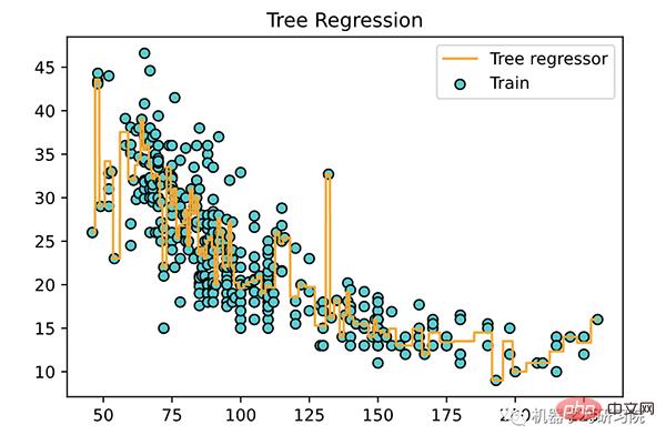
关于决策树的几个关键点：

易于理解和解释，并且决策树可以被可视化显示。
适用于离散值和连续值。
使用 DT预测数据的成本是训练树的训练数据对数量的对数。
决策树的预测既不平滑也不连续（显示为分段常数近似值，如上图所示）。

5. 随机森林回归

一般地，随机森林回归与决策树回归非常相似，它是一个元估计器，在数据集的各种子样本集上拟合许多决策树，并使用平均方法来提高预测准确性和控制过拟合。

随机森林回归器在回归中的性能可能比决策树好，也可能不比决策树好（虽然它通常在分类中表现更好），因为树构造算法本质上存在微妙的过度拟合-欠拟合权衡。

随机森林回归很常见，以至于Scikit-learn内置了RandomForestRegressor. 首先，我们需要创建一个RandomForestRegressor具有指定数量估计器的对象，如下所示：

<span style="color: rgb(215, 58, 73); margin: 0px; padding: 0px; background: none 0% 0% / auto repeat scroll padding-box border-box rgba(0, 0, 0, 0);">from</span> <span style="color: rgb(89, 89, 89); margin: 0px; padding: 0px; background: none 0% 0% / auto repeat scroll padding-box border-box rgba(0, 0, 0, 0);">sklearn</span>.<span style="color: rgb(0, 92, 197); margin: 0px; padding: 0px; background: none 0% 0% / auto repeat scroll padding-box border-box rgba(0, 0, 0, 0);">ensemble</span> <span style="color: rgb(215, 58, 73); margin: 0px; padding: 0px; background: none 0% 0% / auto repeat scroll padding-box border-box rgba(0, 0, 0, 0);">import</span> <span style="color: rgb(89, 89, 89); margin: 0px; padding: 0px; background: none 0% 0% / auto repeat scroll padding-box border-box rgba(0, 0, 0, 0);">RandomForestRegressor</span><br><span style="color: rgb(89, 89, 89); margin: 0px; padding: 0px; background: none 0% 0% / auto repeat scroll padding-box border-box rgba(0, 0, 0, 0);">forest_regressor</span> <span style="color: rgb(215, 58, 73); margin: 0px; padding: 0px; background: none 0% 0% / auto repeat scroll padding-box border-box rgba(0, 0, 0, 0);">=</span> <span style="color: rgb(89, 89, 89); margin: 0px; padding: 0px; background: none 0% 0% / auto repeat scroll padding-box border-box rgba(0, 0, 0, 0);">RandomForestRegressor</span>(<br><span style="color: rgb(89, 89, 89); margin: 0px; padding: 0px; background: none 0% 0% / auto repeat scroll padding-box border-box rgba(0, 0, 0, 0);">n_estimators</span> <span style="color: rgb(215, 58, 73); margin: 0px; padding: 0px; background: none 0% 0% / auto repeat scroll padding-box border-box rgba(0, 0, 0, 0);">=</span> <span style="color: rgb(0, 92, 197); margin: 0px; padding: 0px; background: none 0% 0% / auto repeat scroll padding-box border-box rgba(0, 0, 0, 0);">300</span>,<br><span style="color: rgb(89, 89, 89); margin: 0px; padding: 0px; background: none 0% 0% / auto repeat scroll padding-box border-box rgba(0, 0, 0, 0);">random_state</span> <span style="color: rgb(215, 58, 73); margin: 0px; padding: 0px; background: none 0% 0% / auto repeat scroll padding-box border-box rgba(0, 0, 0, 0);">=</span> <span style="color: rgb(0, 92, 197); margin: 0px; padding: 0px; background: none 0% 0% / auto repeat scroll padding-box border-box rgba(0, 0, 0, 0);">0</span><br>)<br><span style="color: rgb(89, 89, 89); margin: 0px; padding: 0px; background: none 0% 0% / auto repeat scroll padding-box border-box rgba(0, 0, 0, 0);">forest_regressor</span>.<span style="color: rgb(0, 92, 197); margin: 0px; padding: 0px; background: none 0% 0% / auto repeat scroll padding-box border-box rgba(0, 0, 0, 0);">fit</span>(<span style="color: rgb(89, 89, 89); margin: 0px; padding: 0px; background: none 0% 0% / auto repeat scroll padding-box border-box rgba(0, 0, 0, 0);">X</span>, <span style="color: rgb(89, 89, 89); margin: 0px; padding: 0px; background: none 0% 0% / auto repeat scroll padding-box border-box rgba(0, 0, 0, 0);">y</span>.<span style="color: rgb(0, 92, 197); margin: 0px; padding: 0px; background: none 0% 0% / auto repeat scroll padding-box border-box rgba(0, 0, 0, 0);">ravel</span>())<br>

Copy after login

下面使用训练好的模型，绘制一条拟合曲线。

<span style="color: rgb(89, 89, 89); margin: 0px; padding: 0px; background: none 0% 0% / auto repeat scroll padding-box border-box rgba(0, 0, 0, 0);">X_grid</span> <span style="color: rgb(215, 58, 73); margin: 0px; padding: 0px; background: none 0% 0% / auto repeat scroll padding-box border-box rgba(0, 0, 0, 0);">=</span> <span style="color: rgb(89, 89, 89); margin: 0px; padding: 0px; background: none 0% 0% / auto repeat scroll padding-box border-box rgba(0, 0, 0, 0);">np</span>.<span style="color: rgb(0, 92, 197); margin: 0px; padding: 0px; background: none 0% 0% / auto repeat scroll padding-box border-box rgba(0, 0, 0, 0);">arange</span>(<span style="color: rgb(111, 66, 193); margin: 0px; padding: 0px; background: none 0% 0% / auto repeat scroll padding-box border-box rgba(0, 0, 0, 0);">min</span>(<span style="color: rgb(89, 89, 89); margin: 0px; padding: 0px; background: none 0% 0% / auto repeat scroll padding-box border-box rgba(0, 0, 0, 0);">X</span>), <span style="color: rgb(111, 66, 193); margin: 0px; padding: 0px; background: none 0% 0% / auto repeat scroll padding-box border-box rgba(0, 0, 0, 0);">max</span>(<span style="color: rgb(89, 89, 89); margin: 0px; padding: 0px; background: none 0% 0% / auto repeat scroll padding-box border-box rgba(0, 0, 0, 0);">X</span>), <span style="color: rgb(0, 92, 197); margin: 0px; padding: 0px; background: none 0% 0% / auto repeat scroll padding-box border-box rgba(0, 0, 0, 0);">0.01</span>)<br><span style="color: rgb(89, 89, 89); margin: 0px; padding: 0px; background: none 0% 0% / auto repeat scroll padding-box border-box rgba(0, 0, 0, 0);">X_grid</span> <span style="color: rgb(215, 58, 73); margin: 0px; padding: 0px; background: none 0% 0% / auto repeat scroll padding-box border-box rgba(0, 0, 0, 0);">=</span> <span style="color: rgb(89, 89, 89); margin: 0px; padding: 0px; background: none 0% 0% / auto repeat scroll padding-box border-box rgba(0, 0, 0, 0);">X_grid</span>.<span style="color: rgb(0, 92, 197); margin: 0px; padding: 0px; background: none 0% 0% / auto repeat scroll padding-box border-box rgba(0, 0, 0, 0);">reshape</span>(<span style="color: rgb(111, 66, 193); margin: 0px; padding: 0px; background: none 0% 0% / auto repeat scroll padding-box border-box rgba(0, 0, 0, 0);">len</span>(<span style="color: rgb(89, 89, 89); margin: 0px; padding: 0px; background: none 0% 0% / auto repeat scroll padding-box border-box rgba(0, 0, 0, 0);">X_grid</span>), <span style="color: rgb(0, 92, 197); margin: 0px; padding: 0px; background: none 0% 0% / auto repeat scroll padding-box border-box rgba(0, 0, 0, 0);">1</span>)<br><span style="color: rgb(89, 89, 89); margin: 0px; padding: 0px; background: none 0% 0% / auto repeat scroll padding-box border-box rgba(0, 0, 0, 0);">plt</span>.<span style="color: rgb(0, 92, 197); margin: 0px; padding: 0px; background: none 0% 0% / auto repeat scroll padding-box border-box rgba(0, 0, 0, 0);">scatter</span>(<span style="color: rgb(89, 89, 89); margin: 0px; padding: 0px; background: none 0% 0% / auto repeat scroll padding-box border-box rgba(0, 0, 0, 0);">X</span>, <span style="color: rgb(89, 89, 89); margin: 0px; padding: 0px; background: none 0% 0% / auto repeat scroll padding-box border-box rgba(0, 0, 0, 0);">y</span>, <span style="color: rgb(89, 89, 89); margin: 0px; padding: 0px; background: none 0% 0% / auto repeat scroll padding-box border-box rgba(0, 0, 0, 0);">color</span><span style="color: rgb(215, 58, 73); margin: 0px; padding: 0px; background: none 0% 0% / auto repeat scroll padding-box border-box rgba(0, 0, 0, 0);">=</span><span style="color: rgb(102, 153, 0); margin: 0px; padding: 0px; background: none 0% 0% / auto repeat scroll padding-box border-box rgba(0, 0, 0, 0);">'DarkTurquoise'</span>,<br><span style="color: rgb(89, 89, 89); margin: 0px; padding: 0px; background: none 0% 0% / auto repeat scroll padding-box border-box rgba(0, 0, 0, 0);">edgecolors</span><span style="color: rgb(215, 58, 73); margin: 0px; padding: 0px; background: none 0% 0% / auto repeat scroll padding-box border-box rgba(0, 0, 0, 0);">=</span><span style="color: rgb(102, 153, 0); margin: 0px; padding: 0px; background: none 0% 0% / auto repeat scroll padding-box border-box rgba(0, 0, 0, 0);">'black'</span>, <span style="color: rgb(89, 89, 89); margin: 0px; padding: 0px; background: none 0% 0% / auto repeat scroll padding-box border-box rgba(0, 0, 0, 0);">label</span><span style="color: rgb(215, 58, 73); margin: 0px; padding: 0px; background: none 0% 0% / auto repeat scroll padding-box border-box rgba(0, 0, 0, 0);">=</span><span style="color: rgb(102, 153, 0); margin: 0px; padding: 0px; background: none 0% 0% / auto repeat scroll padding-box border-box rgba(0, 0, 0, 0);">'Train'</span>)<br><span style="color: rgb(89, 89, 89); margin: 0px; padding: 0px; background: none 0% 0% / auto repeat scroll padding-box border-box rgba(0, 0, 0, 0);">plt</span>.<span style="color: rgb(0, 92, 197); margin: 0px; padding: 0px; background: none 0% 0% / auto repeat scroll padding-box border-box rgba(0, 0, 0, 0);">plot</span>(<span style="color: rgb(89, 89, 89); margin: 0px; padding: 0px; background: none 0% 0% / auto repeat scroll padding-box border-box rgba(0, 0, 0, 0);">X_grid</span>, <span style="color: rgb(89, 89, 89); margin: 0px; padding: 0px; background: none 0% 0% / auto repeat scroll padding-box border-box rgba(0, 0, 0, 0);">forest_regressor</span>.<span style="color: rgb(0, 92, 197); margin: 0px; padding: 0px; background: none 0% 0% / auto repeat scroll padding-box border-box rgba(0, 0, 0, 0);">predict</span>(<span style="color: rgb(89, 89, 89); margin: 0px; padding: 0px; background: none 0% 0% / auto repeat scroll padding-box border-box rgba(0, 0, 0, 0);">X_grid</span>),<br> <span style="color: rgb(89, 89, 89); margin: 0px; padding: 0px; background: none 0% 0% / auto repeat scroll padding-box border-box rgba(0, 0, 0, 0);">color</span><span style="color: rgb(215, 58, 73); margin: 0px; padding: 0px; background: none 0% 0% / auto repeat scroll padding-box border-box rgba(0, 0, 0, 0);">=</span><span style="color: rgb(102, 153, 0); margin: 0px; padding: 0px; background: none 0% 0% / auto repeat scroll padding-box border-box rgba(0, 0, 0, 0);">'orange'</span>, <span style="color: rgb(89, 89, 89); margin: 0px; padding: 0px; background: none 0% 0% / auto repeat scroll padding-box border-box rgba(0, 0, 0, 0);">label</span><span style="color: rgb(215, 58, 73); margin: 0px; padding: 0px; background: none 0% 0% / auto repeat scroll padding-box border-box rgba(0, 0, 0, 0);">=</span><span style="color: rgb(102, 153, 0); margin: 0px; padding: 0px; background: none 0% 0% / auto repeat scroll padding-box border-box rgba(0, 0, 0, 0);">'Random Forest regressor'</span>)<br><span style="color: rgb(89, 89, 89); margin: 0px; padding: 0px; background: none 0% 0% / auto repeat scroll padding-box border-box rgba(0, 0, 0, 0);">plt</span>.<span style="color: rgb(0, 92, 197); margin: 0px; padding: 0px; background: none 0% 0% / auto repeat scroll padding-box border-box rgba(0, 0, 0, 0);">title</span>(<span style="color: rgb(102, 153, 0); margin: 0px; padding: 0px; background: none 0% 0% / auto repeat scroll padding-box border-box rgba(0, 0, 0, 0);">'Random Forest Regression'</span>)<br><span style="color: rgb(89, 89, 89); margin: 0px; padding: 0px; background: none 0% 0% / auto repeat scroll padding-box border-box rgba(0, 0, 0, 0);">plt</span>.<span style="color: rgb(0, 92, 197); margin: 0px; padding: 0px; background: none 0% 0% / auto repeat scroll padding-box border-box rgba(0, 0, 0, 0);">legend</span>()<br><span style="color: rgb(89, 89, 89); margin: 0px; padding: 0px; background: none 0% 0% / auto repeat scroll padding-box border-box rgba(0, 0, 0, 0);">plt</span>.<span style="color: rgb(0, 92, 197); margin: 0px; padding: 0px; background: none 0% 0% / auto repeat scroll padding-box border-box rgba(0, 0, 0, 0);">show</span>()<br>

Copy after login

Summary of nine top-flow regression algorithms and examples

小结

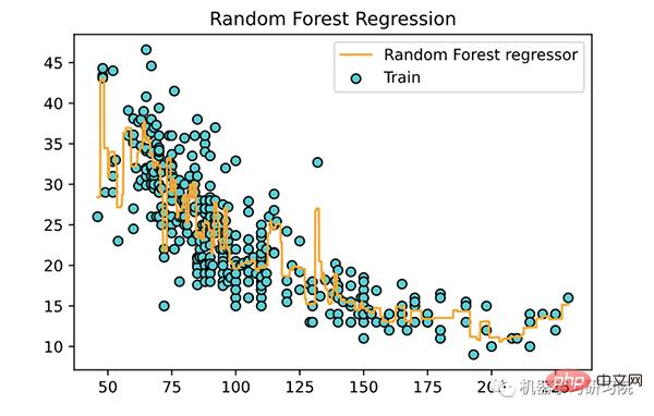
关于随机森林回归的几个关键点：

需要注意减少决策树中的过拟合并提高准确性
它也适用于离散值和连续值
需要大量的计算能力和资源，因为它适合许多决策树来组合它们的输出

6. LASSO 回归

LASSO 回归是使用收缩的线性回归的变体。收缩是数据值向中心点收缩作为均值的过程。这种类型的回归非常适合显示重度多重共线性（特征彼此之间的重度相关性）的模型。

Scikit-learn内置了LassoCV.

<span style="color: rgb(215, 58, 73); margin: 0px; padding: 0px; background: none 0% 0% / auto repeat scroll padding-box border-box rgba(0, 0, 0, 0);">from</span> <span style="color: rgb(89, 89, 89); margin: 0px; padding: 0px; background: none 0% 0% / auto repeat scroll padding-box border-box rgba(0, 0, 0, 0);">sklearn</span>.<span style="color: rgb(0, 92, 197); margin: 0px; padding: 0px; background: none 0% 0% / auto repeat scroll padding-box border-box rgba(0, 0, 0, 0);">linear_model</span> <span style="color: rgb(215, 58, 73); margin: 0px; padding: 0px; background: none 0% 0% / auto repeat scroll padding-box border-box rgba(0, 0, 0, 0);">import</span> <span style="color: rgb(89, 89, 89); margin: 0px; padding: 0px; background: none 0% 0% / auto repeat scroll padding-box border-box rgba(0, 0, 0, 0);">LassoCV</span><br><span style="color: rgb(89, 89, 89); margin: 0px; padding: 0px; background: none 0% 0% / auto repeat scroll padding-box border-box rgba(0, 0, 0, 0);">lasso</span> <span style="color: rgb(215, 58, 73); margin: 0px; padding: 0px; background: none 0% 0% / auto repeat scroll padding-box border-box rgba(0, 0, 0, 0);">=</span> <span style="color: rgb(89, 89, 89); margin: 0px; padding: 0px; background: none 0% 0% / auto repeat scroll padding-box border-box rgba(0, 0, 0, 0);">LassoCV</span>()<br><span style="color: rgb(89, 89, 89); margin: 0px; padding: 0px; background: none 0% 0% / auto repeat scroll padding-box border-box rgba(0, 0, 0, 0);">lasso</span>.<span style="color: rgb(0, 92, 197); margin: 0px; padding: 0px; background: none 0% 0% / auto repeat scroll padding-box border-box rgba(0, 0, 0, 0);">fit</span>(<span style="color: rgb(89, 89, 89); margin: 0px; padding: 0px; background: none 0% 0% / auto repeat scroll padding-box border-box rgba(0, 0, 0, 0);">X</span>, <span style="color: rgb(89, 89, 89); margin: 0px; padding: 0px; background: none 0% 0% / auto repeat scroll padding-box border-box rgba(0, 0, 0, 0);">y</span>.<span style="color: rgb(0, 92, 197); margin: 0px; padding: 0px; background: none 0% 0% / auto repeat scroll padding-box border-box rgba(0, 0, 0, 0);">ravel</span>())<br>

Copy after login

下面使用训练好的模型，绘制一条拟合曲线。

<span style="color: rgb(89, 89, 89); margin: 0px; padding: 0px; background: none 0% 0% / auto repeat scroll padding-box border-box rgba(0, 0, 0, 0);">plt</span>.<span style="color: rgb(0, 92, 197); margin: 0px; padding: 0px; background: none 0% 0% / auto repeat scroll padding-box border-box rgba(0, 0, 0, 0);">scatter</span>(<span style="color: rgb(89, 89, 89); margin: 0px; padding: 0px; background: none 0% 0% / auto repeat scroll padding-box border-box rgba(0, 0, 0, 0);">X</span>, <span style="color: rgb(89, 89, 89); margin: 0px; padding: 0px; background: none 0% 0% / auto repeat scroll padding-box border-box rgba(0, 0, 0, 0);">y</span>, <span style="color: rgb(89, 89, 89); margin: 0px; padding: 0px; background: none 0% 0% / auto repeat scroll padding-box border-box rgba(0, 0, 0, 0);">color</span><span style="color: rgb(215, 58, 73); margin: 0px; padding: 0px; background: none 0% 0% / auto repeat scroll padding-box border-box rgba(0, 0, 0, 0);">=</span><span style="color: rgb(102, 153, 0); margin: 0px; padding: 0px; background: none 0% 0% / auto repeat scroll padding-box border-box rgba(0, 0, 0, 0);">'teal'</span>, <span style="color: rgb(89, 89, 89); margin: 0px; padding: 0px; background: none 0% 0% / auto repeat scroll padding-box border-box rgba(0, 0, 0, 0);">edgecolors</span><span style="color: rgb(215, 58, 73); margin: 0px; padding: 0px; background: none 0% 0% / auto repeat scroll padding-box border-box rgba(0, 0, 0, 0);">=</span><span style="color: rgb(102, 153, 0); margin: 0px; padding: 0px; background: none 0% 0% / auto repeat scroll padding-box border-box rgba(0, 0, 0, 0);">'black'</span>,<br><span style="color: rgb(89, 89, 89); margin: 0px; padding: 0px; background: none 0% 0% / auto repeat scroll padding-box border-box rgba(0, 0, 0, 0);">label</span><span style="color: rgb(215, 58, 73); margin: 0px; padding: 0px; background: none 0% 0% / auto repeat scroll padding-box border-box rgba(0, 0, 0, 0);">=</span><span style="color: rgb(102, 153, 0); margin: 0px; padding: 0px; background: none 0% 0% / auto repeat scroll padding-box border-box rgba(0, 0, 0, 0);">'Actual observation points'</span>)<br><span style="color: rgb(89, 89, 89); margin: 0px; padding: 0px; background: none 0% 0% / auto repeat scroll padding-box border-box rgba(0, 0, 0, 0);">plt</span>.<span style="color: rgb(0, 92, 197); margin: 0px; padding: 0px; background: none 0% 0% / auto repeat scroll padding-box border-box rgba(0, 0, 0, 0);">plot</span>(<span style="color: rgb(89, 89, 89); margin: 0px; padding: 0px; background: none 0% 0% / auto repeat scroll padding-box border-box rgba(0, 0, 0, 0);">X</span>, <span style="color: rgb(89, 89, 89); margin: 0px; padding: 0px; background: none 0% 0% / auto repeat scroll padding-box border-box rgba(0, 0, 0, 0);">lasso</span>.<span style="color: rgb(0, 92, 197); margin: 0px; padding: 0px; background: none 0% 0% / auto repeat scroll padding-box border-box rgba(0, 0, 0, 0);">predict</span>(<span style="color: rgb(89, 89, 89); margin: 0px; padding: 0px; background: none 0% 0% / auto repeat scroll padding-box border-box rgba(0, 0, 0, 0);">X</span>), <span style="color: rgb(89, 89, 89); margin: 0px; padding: 0px; background: none 0% 0% / auto repeat scroll padding-box border-box rgba(0, 0, 0, 0);">color</span><span style="color: rgb(215, 58, 73); margin: 0px; padding: 0px; background: none 0% 0% / auto repeat scroll padding-box border-box rgba(0, 0, 0, 0);">=</span><span style="color: rgb(102, 153, 0); margin: 0px; padding: 0px; background: none 0% 0% / auto repeat scroll padding-box border-box rgba(0, 0, 0, 0);">'orange'</span>,<br> <span style="color: rgb(89, 89, 89); margin: 0px; padding: 0px; background: none 0% 0% / auto repeat scroll padding-box border-box rgba(0, 0, 0, 0);">label</span><span style="color: rgb(215, 58, 73); margin: 0px; padding: 0px; background: none 0% 0% / auto repeat scroll padding-box border-box rgba(0, 0, 0, 0);">=</span><span style="color: rgb(102, 153, 0); margin: 0px; padding: 0px; background: none 0% 0% / auto repeat scroll padding-box border-box rgba(0, 0, 0, 0);">'LASSO regressor'</span>)<br><span style="color: rgb(89, 89, 89); margin: 0px; padding: 0px; background: none 0% 0% / auto repeat scroll padding-box border-box rgba(0, 0, 0, 0);">plt</span>.<span style="color: rgb(0, 92, 197); margin: 0px; padding: 0px; background: none 0% 0% / auto repeat scroll padding-box border-box rgba(0, 0, 0, 0);">title</span>(<span style="color: rgb(102, 153, 0); margin: 0px; padding: 0px; background: none 0% 0% / auto repeat scroll padding-box border-box rgba(0, 0, 0, 0);">'LASSO Regression'</span>)<br><span style="color: rgb(89, 89, 89); margin: 0px; padding: 0px; background: none 0% 0% / auto repeat scroll padding-box border-box rgba(0, 0, 0, 0);">plt</span>.<span style="color: rgb(0, 92, 197); margin: 0px; padding: 0px; background: none 0% 0% / auto repeat scroll padding-box border-box rgba(0, 0, 0, 0);">legend</span>()<br><span style="color: rgb(89, 89, 89); margin: 0px; padding: 0px; background: none 0% 0% / auto repeat scroll padding-box border-box rgba(0, 0, 0, 0);">plt</span>.<span style="color: rgb(0, 92, 197); margin: 0px; padding: 0px; background: none 0% 0% / auto repeat scroll padding-box border-box rgba(0, 0, 0, 0);">show</span>()<br>

Copy after login

Summary of nine top-flow regression algorithms and examples

小结

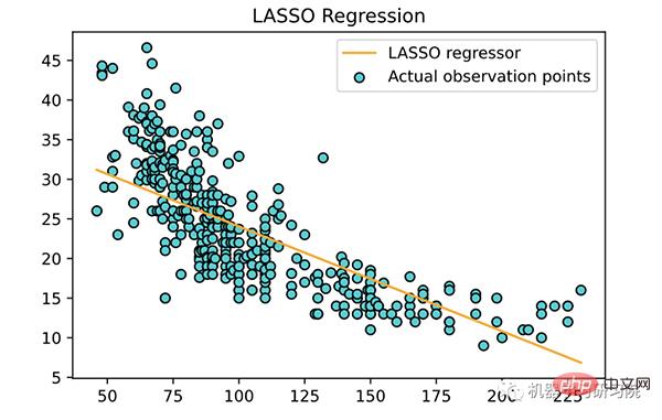
关于套索回归的几点：

它最常用于消除自动化变量和选择特征。
它非常适合显示严重多重共线性（特征彼此高度相关）的模型。
LASSO 回归利用 L1 正则化
LASSO 回归被认为比 Ridge 更好，因为它只选择一些特征并将其他特征的系数降低到零。

7. 岭回归

岭回归与 LASSO 回归非常相似，因为这两种技术都使用收缩。Ridge 回归和 LASSO 回归都非常适合显示重度多重共线性（特征彼此之间的高度相关性）的模型。它们之间的主要区别在于 Ridge 使用 L2 正则化，这意味着没有一个系数像在 LASSO 回归中那样变为零（而是接近零）。

Scikit-learn内置了RidgeCV.

<span style="color: rgb(215, 58, 73); margin: 0px; padding: 0px; background: none 0% 0% / auto repeat scroll padding-box border-box rgba(0, 0, 0, 0);">from</span> <span style="color: rgb(89, 89, 89); margin: 0px; padding: 0px; background: none 0% 0% / auto repeat scroll padding-box border-box rgba(0, 0, 0, 0);">sklearn</span>.<span style="color: rgb(0, 92, 197); margin: 0px; padding: 0px; background: none 0% 0% / auto repeat scroll padding-box border-box rgba(0, 0, 0, 0);">linear_model</span> <span style="color: rgb(215, 58, 73); margin: 0px; padding: 0px; background: none 0% 0% / auto repeat scroll padding-box border-box rgba(0, 0, 0, 0);">import</span> <span style="color: rgb(89, 89, 89); margin: 0px; padding: 0px; background: none 0% 0% / auto repeat scroll padding-box border-box rgba(0, 0, 0, 0);">RidgeCV</span><br><span style="color: rgb(89, 89, 89); margin: 0px; padding: 0px; background: none 0% 0% / auto repeat scroll padding-box border-box rgba(0, 0, 0, 0);">ridge</span> <span style="color: rgb(215, 58, 73); margin: 0px; padding: 0px; background: none 0% 0% / auto repeat scroll padding-box border-box rgba(0, 0, 0, 0);">=</span> <span style="color: rgb(89, 89, 89); margin: 0px; padding: 0px; background: none 0% 0% / auto repeat scroll padding-box border-box rgba(0, 0, 0, 0);">RidgeCV</span>()<br><span style="color: rgb(89, 89, 89); margin: 0px; padding: 0px; background: none 0% 0% / auto repeat scroll padding-box border-box rgba(0, 0, 0, 0);">ridge</span>.<span style="color: rgb(0, 92, 197); margin: 0px; padding: 0px; background: none 0% 0% / auto repeat scroll padding-box border-box rgba(0, 0, 0, 0);">fit</span>(<span style="color: rgb(89, 89, 89); margin: 0px; padding: 0px; background: none 0% 0% / auto repeat scroll padding-box border-box rgba(0, 0, 0, 0);">X</span>, <span style="color: rgb(89, 89, 89); margin: 0px; padding: 0px; background: none 0% 0% / auto repeat scroll padding-box border-box rgba(0, 0, 0, 0);">y</span>)<br>

Copy after login

下面使用训练好的模型，绘制一条拟合曲线。

<span style="color: rgb(89, 89, 89); margin: 0px; padding: 0px; background: none 0% 0% / auto repeat scroll padding-box border-box rgba(0, 0, 0, 0);">plt</span>.<span style="color: rgb(0, 92, 197); margin: 0px; padding: 0px; background: none 0% 0% / auto repeat scroll padding-box border-box rgba(0, 0, 0, 0);">scatter</span>(<span style="color: rgb(89, 89, 89); margin: 0px; padding: 0px; background: none 0% 0% / auto repeat scroll padding-box border-box rgba(0, 0, 0, 0);">X</span>, <span style="color: rgb(89, 89, 89); margin: 0px; padding: 0px; background: none 0% 0% / auto repeat scroll padding-box border-box rgba(0, 0, 0, 0);">y</span>, <span style="color: rgb(89, 89, 89); margin: 0px; padding: 0px; background: none 0% 0% / auto repeat scroll padding-box border-box rgba(0, 0, 0, 0);">color</span><span style="color: rgb(215, 58, 73); margin: 0px; padding: 0px; background: none 0% 0% / auto repeat scroll padding-box border-box rgba(0, 0, 0, 0);">=</span><span style="color: rgb(102, 153, 0); margin: 0px; padding: 0px; background: none 0% 0% / auto repeat scroll padding-box border-box rgba(0, 0, 0, 0);">'teal'</span>, <span style="color: rgb(89, 89, 89); margin: 0px; padding: 0px; background: none 0% 0% / auto repeat scroll padding-box border-box rgba(0, 0, 0, 0);">edgecolors</span><span style="color: rgb(215, 58, 73); margin: 0px; padding: 0px; background: none 0% 0% / auto repeat scroll padding-box border-box rgba(0, 0, 0, 0);">=</span><span style="color: rgb(102, 153, 0); margin: 0px; padding: 0px; background: none 0% 0% / auto repeat scroll padding-box border-box rgba(0, 0, 0, 0);">'black'</span>,<br><span style="color: rgb(89, 89, 89); margin: 0px; padding: 0px; background: none 0% 0% / auto repeat scroll padding-box border-box rgba(0, 0, 0, 0);">label</span><span style="color: rgb(215, 58, 73); margin: 0px; padding: 0px; background: none 0% 0% / auto repeat scroll padding-box border-box rgba(0, 0, 0, 0);">=</span><span style="color: rgb(102, 153, 0); margin: 0px; padding: 0px; background: none 0% 0% / auto repeat scroll padding-box border-box rgba(0, 0, 0, 0);">'Train'</span>)<br><span style="color: rgb(89, 89, 89); margin: 0px; padding: 0px; background: none 0% 0% / auto repeat scroll padding-box border-box rgba(0, 0, 0, 0);">plt</span>.<span style="color: rgb(0, 92, 197); margin: 0px; padding: 0px; background: none 0% 0% / auto repeat scroll padding-box border-box rgba(0, 0, 0, 0);">plot</span>(<span style="color: rgb(89, 89, 89); margin: 0px; padding: 0px; background: none 0% 0% / auto repeat scroll padding-box border-box rgba(0, 0, 0, 0);">X</span>, <span style="color: rgb(89, 89, 89); margin: 0px; padding: 0px; background: none 0% 0% / auto repeat scroll padding-box border-box rgba(0, 0, 0, 0);">ridge</span>.<span style="color: rgb(0, 92, 197); margin: 0px; padding: 0px; background: none 0% 0% / auto repeat scroll padding-box border-box rgba(0, 0, 0, 0);">predict</span>(<span style="color: rgb(89, 89, 89); margin: 0px; padding: 0px; background: none 0% 0% / auto repeat scroll padding-box border-box rgba(0, 0, 0, 0);">X</span>), <span style="color: rgb(89, 89, 89); margin: 0px; padding: 0px; background: none 0% 0% / auto repeat scroll padding-box border-box rgba(0, 0, 0, 0);">color</span><span style="color: rgb(215, 58, 73); margin: 0px; padding: 0px; background: none 0% 0% / auto repeat scroll padding-box border-box rgba(0, 0, 0, 0);">=</span><span style="color: rgb(102, 153, 0); margin: 0px; padding: 0px; background: none 0% 0% / auto repeat scroll padding-box border-box rgba(0, 0, 0, 0);">'orange'</span>,<br> <span style="color: rgb(89, 89, 89); margin: 0px; padding: 0px; background: none 0% 0% / auto repeat scroll padding-box border-box rgba(0, 0, 0, 0);">label</span><span style="color: rgb(215, 58, 73); margin: 0px; padding: 0px; background: none 0% 0% / auto repeat scroll padding-box border-box rgba(0, 0, 0, 0);">=</span><span style="color: rgb(102, 153, 0); margin: 0px; padding: 0px; background: none 0% 0% / auto repeat scroll padding-box border-box rgba(0, 0, 0, 0);">'Ridge regressor'</span>)<br><span style="color: rgb(89, 89, 89); margin: 0px; padding: 0px; background: none 0% 0% / auto repeat scroll padding-box border-box rgba(0, 0, 0, 0);">plt</span>.<span style="color: rgb(0, 92, 197); margin: 0px; padding: 0px; background: none 0% 0% / auto repeat scroll padding-box border-box rgba(0, 0, 0, 0);">title</span>(<span style="color: rgb(102, 153, 0); margin: 0px; padding: 0px; background: none 0% 0% / auto repeat scroll padding-box border-box rgba(0, 0, 0, 0);">'Ridge Regression'</span>)<br><span style="color: rgb(89, 89, 89); margin: 0px; padding: 0px; background: none 0% 0% / auto repeat scroll padding-box border-box rgba(0, 0, 0, 0);">plt</span>.<span style="color: rgb(0, 92, 197); margin: 0px; padding: 0px; background: none 0% 0% / auto repeat scroll padding-box border-box rgba(0, 0, 0, 0);">legend</span>()<br><span style="color: rgb(89, 89, 89); margin: 0px; padding: 0px; background: none 0% 0% / auto repeat scroll padding-box border-box rgba(0, 0, 0, 0);">plt</span>.<span style="color: rgb(0, 92, 197); margin: 0px; padding: 0px; background: none 0% 0% / auto repeat scroll padding-box border-box rgba(0, 0, 0, 0);">show</span>()<br>

Copy after login

Summary of nine top-flow regression algorithms and examples

小结

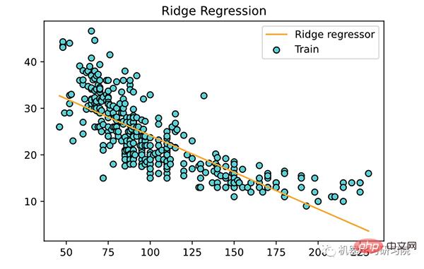
关于岭回归的几个关键点：

它非常适合显示严重多重共线性（特征彼此高度相关）的模型。
岭回归使用 L2 正则化，贡献较小的特征将具有接近零的系数。
由于 L2 正则化的性质，岭回归被认为比 LASSO 差。

8. ElasticNet 回归

ElasticNet 是另一个使用 L1 和 L2 正则化训练的线性回归模型。它是 LASSO 和岭回归技术的混合体，因此它也非常适合显示严重多重共线性（特征彼此高度相关）的模型。

Lasso 和 Ridge 之间权衡的一个实际优势是它允许 Elastic-Net 在旋转时继承一些 Ridge 的稳定性。

Scikit-learn内置了ElasticNetCV模型.

<span style="color: rgb(215, 58, 73); margin: 0px; padding: 0px; background: none 0% 0% / auto repeat scroll padding-box border-box rgba(0, 0, 0, 0);">from</span> <span style="color: rgb(89, 89, 89); margin: 0px; padding: 0px; background: none 0% 0% / auto repeat scroll padding-box border-box rgba(0, 0, 0, 0);">sklearn</span>.<span style="color: rgb(0, 92, 197); margin: 0px; padding: 0px; background: none 0% 0% / auto repeat scroll padding-box border-box rgba(0, 0, 0, 0);">linear_model</span> <span style="color: rgb(215, 58, 73); margin: 0px; padding: 0px; background: none 0% 0% / auto repeat scroll padding-box border-box rgba(0, 0, 0, 0);">import</span> <span style="color: rgb(89, 89, 89); margin: 0px; padding: 0px; background: none 0% 0% / auto repeat scroll padding-box border-box rgba(0, 0, 0, 0);">ElasticNetCV</span><br><span style="color: rgb(89, 89, 89); margin: 0px; padding: 0px; background: none 0% 0% / auto repeat scroll padding-box border-box rgba(0, 0, 0, 0);">elasticNet</span> <span style="color: rgb(215, 58, 73); margin: 0px; padding: 0px; background: none 0% 0% / auto repeat scroll padding-box border-box rgba(0, 0, 0, 0);">=</span> <span style="color: rgb(89, 89, 89); margin: 0px; padding: 0px; background: none 0% 0% / auto repeat scroll padding-box border-box rgba(0, 0, 0, 0);">ElasticNetCV</span>()<br><span style="color: rgb(89, 89, 89); margin: 0px; padding: 0px; background: none 0% 0% / auto repeat scroll padding-box border-box rgba(0, 0, 0, 0);">elasticNet</span>.<span style="color: rgb(0, 92, 197); margin: 0px; padding: 0px; background: none 0% 0% / auto repeat scroll padding-box border-box rgba(0, 0, 0, 0);">fit</span>(<span style="color: rgb(89, 89, 89); margin: 0px; padding: 0px; background: none 0% 0% / auto repeat scroll padding-box border-box rgba(0, 0, 0, 0);">X</span>, <span style="color: rgb(89, 89, 89); margin: 0px; padding: 0px; background: none 0% 0% / auto repeat scroll padding-box border-box rgba(0, 0, 0, 0);">y</span>.<span style="color: rgb(0, 92, 197); margin: 0px; padding: 0px; background: none 0% 0% / auto repeat scroll padding-box border-box rgba(0, 0, 0, 0);">ravel</span>())<br>

Copy after login

下面使用训练好的模型，绘制一条拟合曲线。

<span style="color: rgb(89, 89, 89); margin: 0px; padding: 0px; background: none 0% 0% / auto repeat scroll padding-box border-box rgba(0, 0, 0, 0);">plt</span>.<span style="color: rgb(0, 92, 197); margin: 0px; padding: 0px; background: none 0% 0% / auto repeat scroll padding-box border-box rgba(0, 0, 0, 0);">scatter</span>(<span style="color: rgb(89, 89, 89); margin: 0px; padding: 0px; background: none 0% 0% / auto repeat scroll padding-box border-box rgba(0, 0, 0, 0);">X</span>, <span style="color: rgb(89, 89, 89); margin: 0px; padding: 0px; background: none 0% 0% / auto repeat scroll padding-box border-box rgba(0, 0, 0, 0);">y</span>, <span style="color: rgb(89, 89, 89); margin: 0px; padding: 0px; background: none 0% 0% / auto repeat scroll padding-box border-box rgba(0, 0, 0, 0);">color</span><span style="color: rgb(215, 58, 73); margin: 0px; padding: 0px; background: none 0% 0% / auto repeat scroll padding-box border-box rgba(0, 0, 0, 0);">=</span><span style="color: rgb(102, 153, 0); margin: 0px; padding: 0px; background: none 0% 0% / auto repeat scroll padding-box border-box rgba(0, 0, 0, 0);">'DarkTurquoise'</span>, <span style="color: rgb(89, 89, 89); margin: 0px; padding: 0px; background: none 0% 0% / auto repeat scroll padding-box border-box rgba(0, 0, 0, 0);">edgecolors</span><span style="color: rgb(215, 58, 73); margin: 0px; padding: 0px; background: none 0% 0% / auto repeat scroll padding-box border-box rgba(0, 0, 0, 0);">=</span><span style="color: rgb(102, 153, 0); margin: 0px; padding: 0px; background: none 0% 0% / auto repeat scroll padding-box border-box rgba(0, 0, 0, 0);">'black'</span>, <span style="color: rgb(89, 89, 89); margin: 0px; padding: 0px; background: none 0% 0% / auto repeat scroll padding-box border-box rgba(0, 0, 0, 0);">label</span><span style="color: rgb(215, 58, 73); margin: 0px; padding: 0px; background: none 0% 0% / auto repeat scroll padding-box border-box rgba(0, 0, 0, 0);">=</span><span style="color: rgb(102, 153, 0); margin: 0px; padding: 0px; background: none 0% 0% / auto repeat scroll padding-box border-box rgba(0, 0, 0, 0);">'Train'</span>)<br><span style="color: rgb(89, 89, 89); margin: 0px; padding: 0px; background: none 0% 0% / auto repeat scroll padding-box border-box rgba(0, 0, 0, 0);">plt</span>.<span style="color: rgb(0, 92, 197); margin: 0px; padding: 0px; background: none 0% 0% / auto repeat scroll padding-box border-box rgba(0, 0, 0, 0);">plot</span>(<span style="color: rgb(89, 89, 89); margin: 0px; padding: 0px; background: none 0% 0% / auto repeat scroll padding-box border-box rgba(0, 0, 0, 0);">X</span>, <span style="color: rgb(89, 89, 89); margin: 0px; padding: 0px; background: none 0% 0% / auto repeat scroll padding-box border-box rgba(0, 0, 0, 0);">elasticNet</span>.<span style="color: rgb(0, 92, 197); margin: 0px; padding: 0px; background: none 0% 0% / auto repeat scroll padding-box border-box rgba(0, 0, 0, 0);">predict</span>(<span style="color: rgb(89, 89, 89); margin: 0px; padding: 0px; background: none 0% 0% / auto repeat scroll padding-box border-box rgba(0, 0, 0, 0);">X</span>), <span style="color: rgb(89, 89, 89); margin: 0px; padding: 0px; background: none 0% 0% / auto repeat scroll padding-box border-box rgba(0, 0, 0, 0);">color</span><span style="color: rgb(215, 58, 73); margin: 0px; padding: 0px; background: none 0% 0% / auto repeat scroll padding-box border-box rgba(0, 0, 0, 0);">=</span><span style="color: rgb(102, 153, 0); margin: 0px; padding: 0px; background: none 0% 0% / auto repeat scroll padding-box border-box rgba(0, 0, 0, 0);">'orange'</span>,<span style="color: rgb(89, 89, 89); margin: 0px; padding: 0px; background: none 0% 0% / auto repeat scroll padding-box border-box rgba(0, 0, 0, 0);">label</span><span style="color: rgb(215, 58, 73); margin: 0px; padding: 0px; background: none 0% 0% / auto repeat scroll padding-box border-box rgba(0, 0, 0, 0);">=</span><span style="color: rgb(102, 153, 0); margin: 0px; padding: 0px; background: none 0% 0% / auto repeat scroll padding-box border-box rgba(0, 0, 0, 0);">'ElasticNet regressor'</span>)<br><span style="color: rgb(89, 89, 89); margin: 0px; padding: 0px; background: none 0% 0% / auto repeat scroll padding-box border-box rgba(0, 0, 0, 0);">plt</span>.<span style="color: rgb(0, 92, 197); margin: 0px; padding: 0px; background: none 0% 0% / auto repeat scroll padding-box border-box rgba(0, 0, 0, 0);">title</span>(<span style="color: rgb(102, 153, 0); margin: 0px; padding: 0px; background: none 0% 0% / auto repeat scroll padding-box border-box rgba(0, 0, 0, 0);">'ElasticNet Regression'</span>)<br><span style="color: rgb(89, 89, 89); margin: 0px; padding: 0px; background: none 0% 0% / auto repeat scroll padding-box border-box rgba(0, 0, 0, 0);">plt</span>.<span style="color: rgb(0, 92, 197); margin: 0px; padding: 0px; background: none 0% 0% / auto repeat scroll padding-box border-box rgba(0, 0, 0, 0);">legend</span>()<br><span style="color: rgb(89, 89, 89); margin: 0px; padding: 0px; background: none 0% 0% / auto repeat scroll padding-box border-box rgba(0, 0, 0, 0);">plt</span>.<span style="color: rgb(0, 92, 197); margin: 0px; padding: 0px; background: none 0% 0% / auto repeat scroll padding-box border-box rgba(0, 0, 0, 0);">show</span>()<br>

Copy after login

Summary of nine top-flow regression algorithms and examples

小结

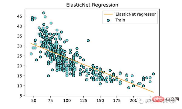
ElasticNet 回归的几个关键点：

ElasticNet 总是优于 LASSO 和 Ridge，因为它解决了两种算法的缺点
ElasticNet 带来了额外的开销，用于确定最佳解决方案的两个 lambda 值。

9. XGBoost 回归

极限梯度提升( XGBoost ) 是梯度提升算法的高效实现。梯度提升是指一类可用于分类或回归问题的集成机器学习算法。

XGBoost是由最初开发的开放源码库tianqi-chen[3]在他的题为“2016论文XGBoost：可扩展树增压系统[4]”。该算法被设计为具有计算效率和高效性。

第一步是安装 XGBoost 库（如果尚未安装）。

<span style="color: rgb(89, 89, 89); margin: 0px; padding: 0px; background: none 0% 0% / auto repeat scroll padding-box border-box rgba(0, 0, 0, 0);">pip</span> <span style="color: rgb(89, 89, 89); margin: 0px; padding: 0px; background: none 0% 0% / auto repeat scroll padding-box border-box rgba(0, 0, 0, 0);">install</span> <span style="color: rgb(89, 89, 89); margin: 0px; padding: 0px; background: none 0% 0% / auto repeat scroll padding-box border-box rgba(0, 0, 0, 0);">xgboost</span><br>

Copy after login

可以通过创建以下实例来定义 XGBoost 模型XGBRegressor：

<span style="color: rgb(215, 58, 73); margin: 0px; padding: 0px; background: none 0% 0% / auto repeat scroll padding-box border-box rgba(0, 0, 0, 0);">from</span> <span style="color: rgb(89, 89, 89); margin: 0px; padding: 0px; background: none 0% 0% / auto repeat scroll padding-box border-box rgba(0, 0, 0, 0);">xgboost</span> <span style="color: rgb(215, 58, 73); margin: 0px; padding: 0px; background: none 0% 0% / auto repeat scroll padding-box border-box rgba(0, 0, 0, 0);">import</span> <span style="color: rgb(89, 89, 89); margin: 0px; padding: 0px; background: none 0% 0% / auto repeat scroll padding-box border-box rgba(0, 0, 0, 0);">XGBRegressor</span><br><span style="color: rgb(106, 115, 125); margin: 0px; padding: 0px; background: none 0% 0% / auto repeat scroll padding-box border-box rgba(0, 0, 0, 0);"># create an xgboost regression model</span><br><span style="color: rgb(89, 89, 89); margin: 0px; padding: 0px; background: none 0% 0% / auto repeat scroll padding-box border-box rgba(0, 0, 0, 0);">model</span> <span style="color: rgb(215, 58, 73); margin: 0px; padding: 0px; background: none 0% 0% / auto repeat scroll padding-box border-box rgba(0, 0, 0, 0);">=</span> <span style="color: rgb(89, 89, 89); margin: 0px; padding: 0px; background: none 0% 0% / auto repeat scroll padding-box border-box rgba(0, 0, 0, 0);">XGBRegressor</span>(<br><span style="color: rgb(89, 89, 89); margin: 0px; padding: 0px; background: none 0% 0% / auto repeat scroll padding-box border-box rgba(0, 0, 0, 0);">n_estimators</span><span style="color: rgb(215, 58, 73); margin: 0px; padding: 0px; background: none 0% 0% / auto repeat scroll padding-box border-box rgba(0, 0, 0, 0);">=</span><span style="color: rgb(0, 92, 197); margin: 0px; padding: 0px; background: none 0% 0% / auto repeat scroll padding-box border-box rgba(0, 0, 0, 0);">1000</span>,<br><span style="color: rgb(89, 89, 89); margin: 0px; padding: 0px; background: none 0% 0% / auto repeat scroll padding-box border-box rgba(0, 0, 0, 0);">max_depth</span><span style="color: rgb(215, 58, 73); margin: 0px; padding: 0px; background: none 0% 0% / auto repeat scroll padding-box border-box rgba(0, 0, 0, 0);">=</span><span style="color: rgb(0, 92, 197); margin: 0px; padding: 0px; background: none 0% 0% / auto repeat scroll padding-box border-box rgba(0, 0, 0, 0);">7</span>,<br><span style="color: rgb(89, 89, 89); margin: 0px; padding: 0px; background: none 0% 0% / auto repeat scroll padding-box border-box rgba(0, 0, 0, 0);">eta</span><span style="color: rgb(215, 58, 73); margin: 0px; padding: 0px; background: none 0% 0% / auto repeat scroll padding-box border-box rgba(0, 0, 0, 0);">=</span><span style="color: rgb(0, 92, 197); margin: 0px; padding: 0px; background: none 0% 0% / auto repeat scroll padding-box border-box rgba(0, 0, 0, 0);">0.1</span>,<br><span style="color: rgb(89, 89, 89); margin: 0px; padding: 0px; background: none 0% 0% / auto repeat scroll padding-box border-box rgba(0, 0, 0, 0);">subsample</span><span style="color: rgb(215, 58, 73); margin: 0px; padding: 0px; background: none 0% 0% / auto repeat scroll padding-box border-box rgba(0, 0, 0, 0);">=</span><span style="color: rgb(0, 92, 197); margin: 0px; padding: 0px; background: none 0% 0% / auto repeat scroll padding-box border-box rgba(0, 0, 0, 0);">0.7</span>,<br><span style="color: rgb(89, 89, 89); margin: 0px; padding: 0px; background: none 0% 0% / auto repeat scroll padding-box border-box rgba(0, 0, 0, 0);">colsample_bytree</span><span style="color: rgb(215, 58, 73); margin: 0px; padding: 0px; background: none 0% 0% / auto repeat scroll padding-box border-box rgba(0, 0, 0, 0);">=</span><span style="color: rgb(0, 92, 197); margin: 0px; padding: 0px; background: none 0% 0% / auto repeat scroll padding-box border-box rgba(0, 0, 0, 0);">0.8</span>,<br>)<br>

Copy after login

n_estimators：整体中的树木数量，通常会增加，直到看不到进一步的改进。
max_depth：每棵树的最大深度，通常值在 1 到 10 之间。
eta：用于对每个模型进行加权的学习率，通常设置为较小的值，例如 0.3、0.1、0.01 或更小。
subsample：每棵树使用的样本数，设置为0到1之间的值，通常为1.0以使用所有样本。
colsample_bytree：每棵树中使用的特征（列）数，设置为 0 到 1 之间的值，通常为 1.0 以使用所有特征。

下面使用训练好的模型，绘制一条拟合曲线。

<span style="color: rgb(89, 89, 89); margin: 0px; padding: 0px; background: none 0% 0% / auto repeat scroll padding-box border-box rgba(0, 0, 0, 0);">plt</span>.<span style="color: rgb(0, 92, 197); margin: 0px; padding: 0px; background: none 0% 0% / auto repeat scroll padding-box border-box rgba(0, 0, 0, 0);">scatter</span>(<span style="color: rgb(89, 89, 89); margin: 0px; padding: 0px; background: none 0% 0% / auto repeat scroll padding-box border-box rgba(0, 0, 0, 0);">X</span>, <span style="color: rgb(89, 89, 89); margin: 0px; padding: 0px; background: none 0% 0% / auto repeat scroll padding-box border-box rgba(0, 0, 0, 0);">y</span>, <span style="color: rgb(89, 89, 89); margin: 0px; padding: 0px; background: none 0% 0% / auto repeat scroll padding-box border-box rgba(0, 0, 0, 0);">color</span><span style="color: rgb(215, 58, 73); margin: 0px; padding: 0px; background: none 0% 0% / auto repeat scroll padding-box border-box rgba(0, 0, 0, 0);">=</span><span style="color: rgb(102, 153, 0); margin: 0px; padding: 0px; background: none 0% 0% / auto repeat scroll padding-box border-box rgba(0, 0, 0, 0);">'DarkTurquoise'</span>, <span style="color: rgb(89, 89, 89); margin: 0px; padding: 0px; background: none 0% 0% / auto repeat scroll padding-box border-box rgba(0, 0, 0, 0);">edgecolors</span><span style="color: rgb(215, 58, 73); margin: 0px; padding: 0px; background: none 0% 0% / auto repeat scroll padding-box border-box rgba(0, 0, 0, 0);">=</span><span style="color: rgb(102, 153, 0); margin: 0px; padding: 0px; background: none 0% 0% / auto repeat scroll padding-box border-box rgba(0, 0, 0, 0);">'black'</span>, <span style="color: rgb(89, 89, 89); margin: 0px; padding: 0px; background: none 0% 0% / auto repeat scroll padding-box border-box rgba(0, 0, 0, 0);">label</span><span style="color: rgb(215, 58, 73); margin: 0px; padding: 0px; background: none 0% 0% / auto repeat scroll padding-box border-box rgba(0, 0, 0, 0);">=</span><span style="color: rgb(102, 153, 0); margin: 0px; padding: 0px; background: none 0% 0% / auto repeat scroll padding-box border-box rgba(0, 0, 0, 0);">'Train'</span>)<br><span style="color: rgb(89, 89, 89); margin: 0px; padding: 0px; background: none 0% 0% / auto repeat scroll padding-box border-box rgba(0, 0, 0, 0);">plt</span>.<span style="color: rgb(0, 92, 197); margin: 0px; padding: 0px; background: none 0% 0% / auto repeat scroll padding-box border-box rgba(0, 0, 0, 0);">plot</span>(<span style="color: rgb(89, 89, 89); margin: 0px; padding: 0px; background: none 0% 0% / auto repeat scroll padding-box border-box rgba(0, 0, 0, 0);">X</span>, <span style="color: rgb(89, 89, 89); margin: 0px; padding: 0px; background: none 0% 0% / auto repeat scroll padding-box border-box rgba(0, 0, 0, 0);">model</span>.<span style="color: rgb(0, 92, 197); margin: 0px; padding: 0px; background: none 0% 0% / auto repeat scroll padding-box border-box rgba(0, 0, 0, 0);">predict</span>(<span style="color: rgb(89, 89, 89); margin: 0px; padding: 0px; background: none 0% 0% / auto repeat scroll padding-box border-box rgba(0, 0, 0, 0);">X</span>), <span style="color: rgb(89, 89, 89); margin: 0px; padding: 0px; background: none 0% 0% / auto repeat scroll padding-box border-box rgba(0, 0, 0, 0);">color</span><span style="color: rgb(215, 58, 73); margin: 0px; padding: 0px; background: none 0% 0% / auto repeat scroll padding-box border-box rgba(0, 0, 0, 0);">=</span><span style="color: rgb(102, 153, 0); margin: 0px; padding: 0px; background: none 0% 0% / auto repeat scroll padding-box border-box rgba(0, 0, 0, 0);">'orange'</span>,<span style="color: rgb(89, 89, 89); margin: 0px; padding: 0px; background: none 0% 0% / auto repeat scroll padding-box border-box rgba(0, 0, 0, 0);">label</span><span style="color: rgb(215, 58, 73); margin: 0px; padding: 0px; background: none 0% 0% / auto repeat scroll padding-box border-box rgba(0, 0, 0, 0);">=</span><span style="color: rgb(102, 153, 0); margin: 0px; padding: 0px; background: none 0% 0% / auto repeat scroll padding-box border-box rgba(0, 0, 0, 0);">'XGBoost regressor'</span>)<br><span style="color: rgb(89, 89, 89); margin: 0px; padding: 0px; background: none 0% 0% / auto repeat scroll padding-box border-box rgba(0, 0, 0, 0);">plt</span>.<span style="color: rgb(0, 92, 197); margin: 0px; padding: 0px; background: none 0% 0% / auto repeat scroll padding-box border-box rgba(0, 0, 0, 0);">title</span>(<span style="color: rgb(102, 153, 0); margin: 0px; padding: 0px; background: none 0% 0% / auto repeat scroll padding-box border-box rgba(0, 0, 0, 0);">'XGBoost Regression'</span>)<br><span style="color: rgb(89, 89, 89); margin: 0px; padding: 0px; background: none 0% 0% / auto repeat scroll padding-box border-box rgba(0, 0, 0, 0);">plt</span>.<span style="color: rgb(0, 92, 197); margin: 0px; padding: 0px; background: none 0% 0% / auto repeat scroll padding-box border-box rgba(0, 0, 0, 0);">legend</span>()<br><span style="color: rgb(89, 89, 89); margin: 0px; padding: 0px; background: none 0% 0% / auto repeat scroll padding-box border-box rgba(0, 0, 0, 0);">plt</span>.<span style="color: rgb(0, 92, 197); margin: 0px; padding: 0px; background: none 0% 0% / auto repeat scroll padding-box border-box rgba(0, 0, 0, 0);">show</span>()<br>

Copy after login

Summary of nine top-flow regression algorithms and examples

小结

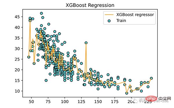
关于 XGBoost 的几个关键点：

XGBoost 在稀疏和非结构化数据上表现不佳。
该算法旨在计算高效且高效，但对于大型数据集而言，训练时间仍然相当长
对异常值很敏感

写在最后

到这里本文就结束啦，本文我们通过使用Scikit-learn和 XGBoost 的动手实践介绍了九种流行的回归算法。在解决实际问题时，可以尝试不同的算法并找到解决实际问题的最佳回归模型。

The above is the detailed content of Summary of nine top-flow regression algorithms and examples. For more information, please follow other related articles on the PHP Chinese website!