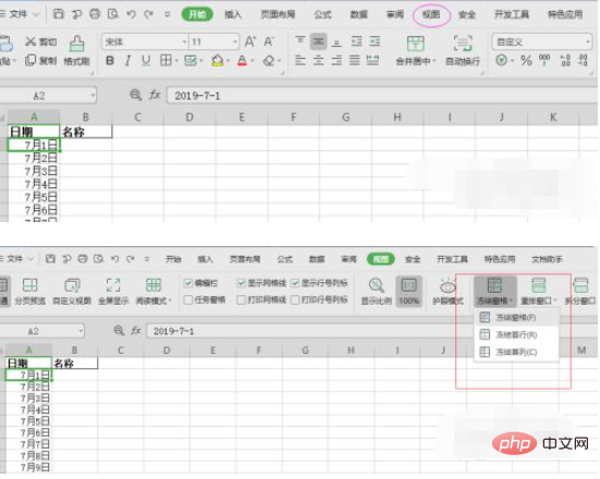
How to freeze selected area in excel

How to freeze the selected area in Excel: First select the position you want to fix; then click "View" on the menu bar at the top of the table, and then click "Freeze Window" below "Freeze Pane" Just click “Form”.

The operating environment of this article: Windows 7 system, Microsoft Office Excel 2010 version, Dell G3 computer.

How to freeze the selected area in Excel:

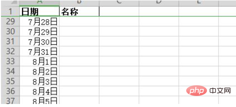
1. First select the position you want to fix, and then click the cursor on the table you want to fix. Below, for example, if I want to fix the first row, then position the cursor at the first grid "A2" of the second row

2, second Click "View" on the menu bar at the top of the table, and then click "Freeze Panes" below "Freeze Panes". You can also press the letter key F to freeze the panes; to cancel, click Unfreeze Panes or press the F key.

3. This way, when there is a lot of data in the table, it will be easier for you to view it

Related learning recommendations:excel basic tutorial

The above is the detailed content of How to freeze selected area in excel. For more information, please follow other related articles on the PHP Chinese website!