How to Use the MAX Function in Excel

The MAX function in Microsoft Excel is a powerful tool used to find the highest numerical value within a specified range or array of numbers. It is commonly used in data analysis and calculations to quickly determine the maximum value in a dataset. Excel efficiently returns the largest number by simply inputting the range or list of values into the MAX function, making it indispensable for tasks requiring quick identification of peak values.

Key Takeaways:

• Excel’s MAX function identifies the highest number in a given range of cells, simplifying data analysis by quickly pinpointing top values.
• Implementing MAX is straightforward—simply select your data range and let the function do the work by typing =MAX( followed by the range and ).
• MAX handles both contiguous and non-contiguous data, making it adaptable for various scenarios, from simple ranges to complex nested functions.
• Combine MAX with other Excel functions like IF, INDEX, and MATCH to perform more sophisticated analyses, such as finding the highest value meeting specific criteria or locating its position within a dataset.
• MAX proves invaluable in practical situations like sales analysis or academic grading, where identifying the highest value quickly highlights success or areas for improvement.

Introduction to Excel’s Mighty MAX Function

Understanding the Basics of MAX

When you dive into Excel’s toolbox, the MAX function emerges as one of the basics that is indispensable. Simply put, MAX is your go-to when you need to identify the largest number within a range of cells. It effortlessly sifts through rows and columns, bringing the highest value to your attention.

Imagine being able to pinpoint the top sales figure or the maximum value in a series of test scores with just a few clicks. That’s the kind of straightforward efficiency MAX brings to your spreadsheets, helping you to summarize data instantly without the hassle of manual comparison.

Step-by-Step Guide to Implementing MAX in Your Workbook

Implementing the MAX function in your workbook is like adding a new tool to your belt—one that’s surprisingly easy to use. Here’s a step-by-step guide to help you get started:

STEP 1: Identify the Destination Cell: Click the cell in your workbook where you want the MAX result to appear.

STEP 2: Begin the Formula: Type in =MAX( to initiate the function.

STEP 3: Select Your Data Range: Click and drag to select the cells that contain the numbers you want to evaluate. Your formula should now look similar to =MAX(B2:B21.

STEP 4: Close the Formula: Type ) to close the function.

STEP 5: Execute the Function: Press Enter, and voila, the highest number in your selected range will populate in your chosen cell.

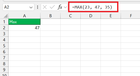
Remember, MAX is flexible. If you need to calculate the maximum value across different, non-adjacent cells or ranges, simply separate them with commas. What makes it powerful is its versatility. You can feed MAX a simple set of static numbers, like =MAX(23, 47, 35).

And if you’re dealing with data scattered across your workbook, MAX doesn’t blink an eye—=MAX(B2, B5, B8) would seamlessly compute the highest value from those individual cells.

As you become more comfortable, you may find creative ways to leverage MAX, such as nesting it within other functions or using it alongside conditional statements for more complex analyses.

Beyond the Basics: Advanced Tips for the MAX Function

Pairing MAX with Other Formulas for Enhanced Analysis

Think of the MAX function as a team player—it pairs beautifully with other Excel formulas to unlock even more powerful and nuanced data analysis. By combining MAX with functions like IF, INDEX, and MATCH, you create an analytical dream team capable of tackling complex problems.

For instance, let’s say you want to identify the highest value that meets a specific condition. Pairing MAX with the IF function allows you to do just that. The formula =MAX(IF(range=criteria, max_range)) filters only the cells that meet your criteria and then determine the highest value among them.

Need to pinpoint the location of your maximum value within a dataset? MAX, meet MATCH. Together, they can find the position of the top value in a range. Start with an INDEX function to retrieve the actual data and then add MATCH into the mix. The final command might look something like this: =INDEX(range, MATCH(MAX(range), range, 0)).

The trick is to think of MAX as your starting point and then layer on additional functions as your analysis requirements grow more sophisticated.

Real-World Examples to Level Up Your MAX Skills

Example Scenarios Where MAX Saves the Day

Sometimes, you only know the true value of a tool when you see it in action. Here are a couple of scenarios where the MAX function becomes indispensable:

• Sales Analysis: Imagine you’re staring down a spreadsheet filled with this quarter’s sales figures from multiple regions. With the MAX function, you can swiftly highlight the region with the top sales, instigating a deeper dive into what’s driving that region’s success and potentially replicating the strategy elsewhere.
• Academic Grading: Teachers can use MAX to quickly pinpoint the highest-scoring student in a particular test, allowing them to recognize outstanding performance or assess the effectiveness of their teaching materials based on the class’s peak scores.

In both cases, MAX does the legwork of sifting through the numbers, letting you focus on the story behind the data, be it a tale of sales triumphs or academic achievement.

Frequently Asked Questions

What is the max function in Excel do?

The MAX function in Excel is designed to calculate and return the highest numeric value within a set of values provided to it. It’s particularly handy when you need to quickly identify the maximum number in a range of cells or array—whether it’s sales figures, scores, temperatures, or any dataset where you need to find the top value.

How to use max function in Excel with multiple conditions?

To use the max function in Excel with multiple conditions, you’d typically combine it with the IF function in an array formula, which you enter by pressing Ctrl Shift Enter. For example, =MAX(IF(condition1, IF(condition2, range))) filters data that meets your criteria and then calculates the maximum value of the filtered set.

Can MAX Function Handle Text and Logical Values?

The standard MAX function in Excel ignores text and logical values (TRUE and FALSE) within a range; it strictly calculates the highest numeric value. For cases where you need to account for logical values in your calculations, consider using the MAXA function, which treats TRUE as 1 and FALSE as 0.

How to Address Errors When Using the MAX Function?

Address errors when using the MAX function by ensuring your data range contains only numeric values, as non-numeric entries cause a #VALUE! error. Use the IFERROR function to manage individual errors, or the AGGSTRUCTURE function to ignore error values within the range during the calculation.

What is the difference between large and max in Excel?

The difference lies in their purpose: the MAX function in Excel finds the largest value in a dataset, while LARGE returns the nth largest value. For instance, while MAX will give you the top sales figure, LARGE lets you identify the second, third, or any specific rank of high values in a range when you specify its position as an additional argument.

The above is the detailed content of How to Use the MAX Function in Excel. For more information, please follow other related articles on the PHP Chinese website!